Page 84 - Classification Parameter Estimation & State Estimation An Engg Approach Using MATLAB

DATA FITTING 73

2ε
ε 2
ρ (ε)
ρ(ε) ε

ε

–σ +σ ε –σ +σ

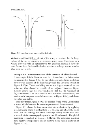
Figure 3.9 A robust error norm and its derivative

derivative e (e) ¼ q e kk =qx of (:) is nearly a constant. But for large
robust
values of e, i.e. for outliers, it becomes nearly zero. Therefore, in a
Gauss–Newton style of optimization, the Jacobian matrix is virtually
zero for outliers. Only residuals that are about as large as or smaller
than that play a role.

Example 3.9 Robust estimation of the diameter of a blood vessel
If in example 3.8 the diameter must be estimated near the bifurcation
(as indicated in Figure 3.8(a) by the white arrows) a large modelling
error occurs because of the branching vessel. See the cross-section in
Figure 3.10(a). These modelling errors are large compared to the
noise and they should be considered as outliers. However, Figure
2
e
3.10(b) shows that the error landscape kk has its minimum at
2
^
D D LS ¼ 0:50 mm. The true value is D ¼ 0:40 mm. Furthermore, the
minimum is less pronounced than the one in Figure 3.8(c), and there-
fore also less stable.
Note also that in Figure 3.10(a) the position found by the LS estimator
is in the middle between the two true positions of the two vessels.
Figure 3.11 shows the improvements that are obtained by applying
a robust error norm. The threshold is selected just above the noise
level. For this setting, the error landscape clearly shows two pro-
nounced minima corresponding to the two blood vessels. The global
^
minimum is reached at D robust ¼ 0:44 mm. The estimated position
D
now clearly corresponds to one of the two blood vessels as shown in
Figure 3.11(a).