Page 90 - Compact Numerical Methods For Computers

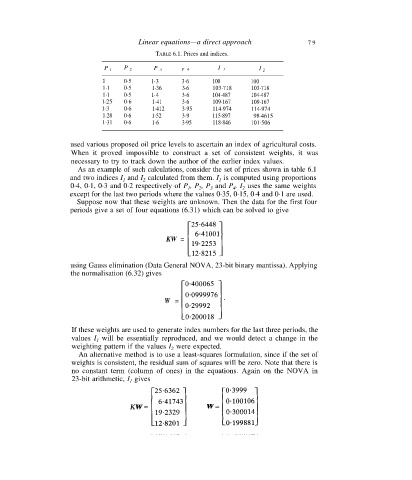
Linear equations—a direct approach 7 9
TABLE 6.1. Prices and indices.

P 1 P 2 P 3 P 4 I 1 I 2
1 0·5 l·3 3·6 100 100
1·1 0·5 1·36 3·6 103·718 103·718
1·l 0·5 l·4 3·6 104·487 104·487
l·25 0·6 1·41 3·6 109·167 109·167
l·3 0·6 1·412 3·95 114·974 114·974
1·28 0·6 1·52 3·9 115·897 98·4615
1·31 0·6 1·6 3·95 118·846 101·506

used various proposed oil price levels to ascertain an index of agricultural costs.
When it proved impossible to construct a set of consistent weights, it was
necessary to try to track down the author of the earlier index values.
As an example of such calculations, consider the set of prices shown in table 6.1
and two indices I and I calculated from them. I is computed using proportions
1
2
1
0·4, 0·1, 0·3 and 0·2 respectively of P , P , P and P . I uses the same weights
1 2 3 4 2
except for the last two periods where the values 0·35, 0·15, 0·4 and 0·1 are used.
Suppose now that these weights are unknown. Then the data for the first four
periods give a set of four equations (6.31) which can be solved to give

KW =

using Gauss elimination (Data General NOVA, 23-bit binary mantissa). Applying
the normalisation (6.32) gives

W =

If these weights are used to generate index numbers for the last three periods, the
values I 1 will be essentially reproduced, and we would detect a change in the
weighting pattern if the values I were expected.
2
An alternative method is to use a least-squares formulation, since if the set of
weights is consistent, the residual sum of squares will be zero. Note that there is
no constant term (column of ones) in the equations. Again on the NOVA in
23-bit arithmetic, I gives
1