Page 99 - Computational Colour Science Using MATLAB

86 CHROMATIC-ADAPTATION TRANSFORMS AND COLOUR APPEARANCE

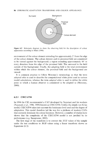
Figure 6.2 Schematic diagram to show the observing field for the description of colour
appearance according to Hunt (1998)

environment of the colour element extending for approximately 28 from the edge
of the colour element. The colour element and its proximal field are considered
to be viewed against the background, a region extending approximately 108 in
every direction from the edge of the proximal field. The surround is the field
outside of the background. Finally, the adapting field is the total environment
within which the colour element, the proximal field and the background are
viewed.
It is common practice to follow Moroney’s terminology so that the term
adopted white is used to describe the computational white point used in various
model calculations, whereas the term adapted white is used to define the white
point to which a human observer is considered to be adapted to (Moroney,
2000).

6.2.1 CIECAT94

In 1994 the CIE recommended a CAT developed by Nayatani and his workers
(Nayatani et al., 1990, 1999) known as CIECAT94. Unlike the simple von Kries
model, CIECAT94 takes into account the luminance level used and the degree of
adaptation. This model therefore led the way for a plethora of modern CATs
that currently dominate the colour literature. However, a number of studies have
shown that the complexity of the CIECAT94 model is not justified by its
performance (e.g. Sueeprasan, 2003).
The first stage of the transform is to convert the XYZ values of the sample
under the test conditions to RGB values using a linear transform shown as
Equations (6.3):