Page 105 - Computational Fluid Dynamics for Engineers
P. 105

3.5  Initial  Conditions                                               91


                                                         100,000

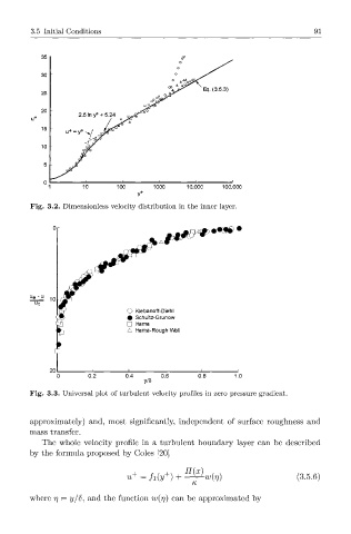
         Fig.  3.2.  Dimensionless  velocity  distribution  in the  inner  layer.


                                                  ^    • • * § > •
                                      *<t*#>


         iie__u  1Q
                                 O  Klebanoff-Diehl
                                 #  Schultz-Grunow
                                 D  Hama
                                 A  Hama-Rough VVall


               0       0.2       0.4     0.6       0.8      1.0
                                     y/8
         Fig.  3.3.  Universal  plot  of turbulent  velocity  profiles  in  zero  pressure  gradient.


         approximately)  and,  most  significantly,  independent  of  surface  roughness  and
         mass  transfer.
            The  whole  velocity  profile  in  a  turbulent  boundary  layer  can  be  described
         by the  formula  proposed  by  Coles  [20]


                                          +
                                 u +  =  h(y )  +  I ^-w{r 1)              (3.5.6)
         where  r)  =  y/8,  and  the  function  w{rj)  can  be  approximated  by
   100   101   102   103   104   105   106   107   108   109   110