Page 217 -

Section 6.4 Image Denoising 185

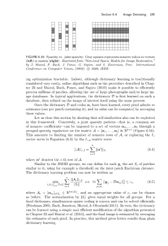
FIGURE 6.16: Sparsity vs. joint sparsity: Gray squares represents nonzero values in vectors
(left)or matrix (right). Reprinted from “Non-local Sparse Models for Image Restoration,”
by J. Mairal, F. Bach, J. Ponce, G. Sapiro, and A. Zisserman, Proc. International
Conference on Computer Vision, (2009). c 2009, IEEE.

ing optimization tractable. Indeed, although dictionary learning is traditionally
considered very costly, online algorithms such as the procedure described in Chap-
ter 22 and Mairal, Bach, Ponce, and Sapiro (2010) make it possible to efficiently
process millions of patches, allowing the use of large photographs and/or large im-
age databases. In typical applications, the dictionary D is first learned on such a
database, then refined on the image of interest itself using the same process.
Once the dictionary D and codes α i have been learned, every pixel admits m
estimates (one per patch containing it), and its value can be computed by averaging
these values.
Let us close this section by showing that self-similarities also can be exploited
in this framework. Concretely, a joint sparsity pattern—that is, a common set
of nonzero coefficients—can be imposed to a set of vectors α 1 ,..., α l through a
grouped-sparsity regularizer on the matrix A =[α 1 ,..., α l ]in R k×l (Figure 6.16).
This amounts to limiting the number of nonzero rows of A, or replacing the 1
vector norm in Equation (6.3) by the 1,2 matrix norm
k

i
||A|| 1,2 = ||α || 2 , (6.4)
i=1
i
where α denotes the i-th row of A.
Similar to the BM3D groups, we can define for each y the set S i of patches
i
similar to it, using for example a threshold on the inter-patch Euclidean distance.
The dictionary learning problem can now be written as
n
||A i || 1,2
2
min s.t. ∀i ||y −Dα ij || ≤ ε i , (6.5)
j
2
(A i ) n i=1 ,D∈C i=1 |S i | j∈S i
∈ R k×|S i | , and an appropriate value of ε i can be chosen
where A i =[α ij ] j∈§ i
as before. The normalization by |S i | gives equal weights for all groups. For a
fixed dictionary, simultaneous sparse coding is convex and can be solved efficiently
(Friedman 2001; Bach, Jenatton, Mairal, & Obozinski 2011). In turn, the dictionary
can be learned using a simple and efficient modification of the algorithm presented
in Chapter 22 and Mairal et al. (2010), and the final image is estimated by averaging
the estimates of each pixel. In practice, this method gives better results than plain
dictionary learning.