Page 624 - Discrete Mathematics and Its Applications

9.4 Closures of Relations 603

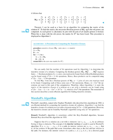
it follows that
⎡ ⎤ ⎡ ⎤ ⎡ ⎤ ⎡ ⎤
1 0 1 1 1 1 1 1 1 1 1 1
M R = ⎣ 0 1 0 ⎦ ∨ 0 1 0 ⎦ ∨ 0 1 0 ⎦ = ⎣ 0 1 0 ⎦ .
∗
⎣
⎣
1 1 0 1 1 1 1 1 1 1 1 1
▲
Theorem 3 can be used as a basis for an algorithm for computing the matrix of the
∗
relation R . To find this matrix, the successive Boolean powers of M R ,uptothe nth power, are
computed. As each power is calculated, its join with the join of all smaller powers is formed.
∗
When this is done with the nth power, the matrix for R has been found. This procedure is
displayed as Algorithm 1.

ALGORITHM 1 A Procedure for Computing the Transitive Closure.

procedure transitive closure (M R : zero–one n × n matrix)
A := M R
B := A
for i := 2 to n
A := A M R
B := B ∨ A
∗
return B{B is the zero–one matrix for R }

We can easily find the number of bit operations used by Algorithm 1 to determine the
[2]
transitive closure of a relation. Computing the Boolean powers M R , M ,..., M [n] requires
R R
thatn − 1Booleanproductsofn × nzero–onematricesbefound.EachoftheseBooleanproducts
2
can be found using n (2n − 1) bit operations. Hence, these products can be computed using
2
n (2n − 1)(n − 1) bit operations.
To find M R from the n Boolean powers of M R , n − 1 joins of zero–one matrices need
∗
2
2
to be found. Computing each of these joins uses n bit operations. Hence, (n − 1)n bit op-
erations are used in this part of the computation. Therefore, when Algorithm 1 is used, the
matrix of the transitive closure of a relation on a set with n elements can be found using
4
3
2
2
n (2n − 1)(n − 1) + (n − 1)n = 2n (n − 1), which is O(n ) bit operations. The remainder of
this section describes a more efficient algorithm for finding transitive closures.
Warshall’s Algorithm
Warshall’s algorithm, named after Stephen Warshall, who described this algorithm in 1960, is
an efficient method for computing the transitive closure of a relation. Algorithm 1 can find the
3
transitive closure of a relation on a set with n elements using 2n (n − 1) bit operations. However,
3
the transitive closure can be found by Warshall’s algorithm using only 2n bit operations.
Remark: Warshall’s algorithm is sometimes called the Roy–Warshall algorithm, because
Bernard Roy described this algorithm in 1959.

Suppose that R is a relation on a set with n elements. Let v 1 , v 2 ,..., v n be an arbitrary
listing of these n elements. The concept of the interior vertices of a path is used in Warshall’s
algorithm. If a, x 1 ,x 2 ,...,x m−1 , b is a path, its interior vertices are x 1 ,x 2 ,...,x m−1 , that
is, all the vertices of the path that occur somewhere other than as the first and last vertices in
the path. For instance, the interior vertices of a path a, c, d, f, g, h, b, j in a directed graph