Page 683 - Discrete Mathematics and Its Applications

662 10 / Graphs

P(0, 0) P(0, 1) P(0, 2) P(0, 3)

P(1, 0) P(1, 1) P(1, 2) P(1, 3)

P(2, 0) P(2, 1) P(2, 2) P(2, 3)

P 1 P 2 P 3 P 4 P 5 P 6 P(3, 0) P(3, 1) P(3, 2) P(3, 3)

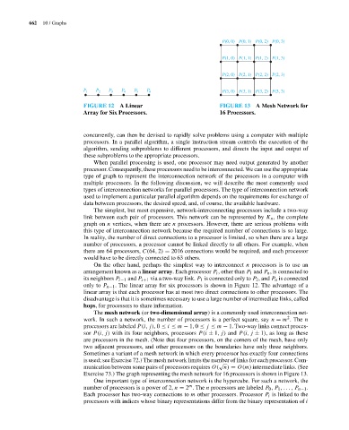
FIGURE 12 A Linear FIGURE 13 A Mesh Network for
Array for Six Processors. 16 Processors.

concurrently, can then be devised to rapidly solve problems using a computer with multiple
processors. In a parallel algorithm, a single instruction stream controls the execution of the
algorithm, sending subproblems to different processors, and directs the input and output of
these subproblems to the appropriate processors.
When parallel processing is used, one processor may need output generated by another
processor. Consequently, these processors need to be interconnected. We can use the appropriate
type of graph to represent the interconnection network of the processors in a computer with
multiple processors. In the following discussion, we will describe the most commonly used
types of interconnection networks for parallel processors. The type of interconnection network
used to implement a particular parallel algorithm depends on the requirements for exchange of
data between processors, the desired speed, and, of course, the available hardware.
The simplest, but most expensive, network-interconnecting processors include a two-way
link between each pair of processors. This network can be represented by K n , the complete
graph on n vertices, when there are n processors. However, there are serious problems with
this type of interconnection network because the required number of connections is so large.
In reality, the number of direct connections to a processor is limited, so when there are a large
number of processors, a processor cannot be linked directly to all others. For example, when
there are 64 processors, C(64, 2) = 2016 connections would be required, and each processor
would have to be directly connected to 63 others.
On the other hand, perhaps the simplest way to interconnect n processors is to use an
arrangement known as a linear array. Each processor P i , other than P 1 and P n , is connected to
its neighbors P i−1 and P i+1 via a two-way link. P 1 is connected only to P 2 , and P n is connected
only to P n−1 . The linear array for six processors is shown in Figure 12. The advantage of a
linear array is that each processor has at most two direct connections to other processors. The
disadvantage is that it is sometimes necessary to use a large number of intermediate links, called
hops, for processors to share information.
The mesh network (or two-dimensional array) is a commonly used interconnection net-
2
work. In such a network, the number of processors is a perfect square, say n = m . The n
processors are labeled P(i, j),0 ≤ i ≤ m − 1, 0 ≤ j ≤ m − 1. Two-way links connect proces-
sor P(i, j) with its four neighbors, processors P(i ± 1,j) and P(i, j ± 1), as long as these
are processors in the mesh. (Note that four processors, on the corners of the mesh, have only
two adjacent processors, and other processors on the boundaries have only three neighbors.
Sometimes a variant of a mesh network in which every processor has exactly four connections
is used; see Exercise 72.) The mesh network limits the number of links for each processor. Com-
√
munication between some pairs of processors requires O( n) = O(m) intermediate links. (See
Exercise 73.) The graph representing the mesh network for 16 processors is shown in Figure 13.
One important type of interconnection network is the hypercube. For such a network, the
m
number of processors is a power of 2, n = 2 . The n processors are labeled P 0 ,P 1 ,...,P n−1 .
Each processor has two-way connections to m other processors. Processor P i is linked to the
processors with indices whose binary representations differ from the binary representation of i