Page 194 -

11-ch04-125-186-9780123814791
3:17 Page 157
HAN
2011/6/1
#33
4.4 Data Warehouse Implementation 157

The compute cube Operator and the Curse
of Dimensionality
One approach to cube computation extends SQL so as to include a compute cube oper-
ator. The compute cube operator computes aggregates over all subsets of the dimensions
specified in the operation. This can require excessive storage space, especially for large
numbers of dimensions. We start with an intuitive look at what is involved in the
efficient computation of data cubes.

Example 4.6 A data cube is a lattice of cuboids. Suppose that you want to create a data cube for
AllElectronics sales that contains the following: city, item, year, and sales in dollars. You
want to be able to analyze the data, with queries such as the following:

“Compute the sum of sales, grouping by city and item.”
“Compute the sum of sales, grouping by city.”
“Compute the sum of sales, grouping by item.”

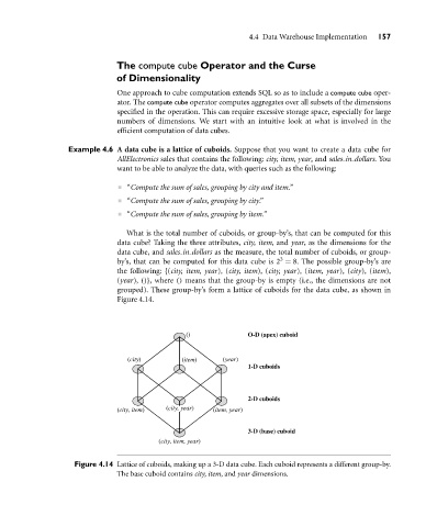
What is the total number of cuboids, or group-by’s, that can be computed for this
data cube? Taking the three attributes, city, item, and year, as the dimensions for the
data cube, and sales in dollars as the measure, the total number of cuboids, or group-
3
by’s, that can be computed for this data cube is 2 = 8. The possible group-by’s are
the following: {(city, item, year), (city, item), (city, year), (item, year), (city), (item),
(year), ()}, where () means that the group-by is empty (i.e., the dimensions are not
grouped). These group-by’s form a lattice of cuboids for the data cube, as shown in
Figure 4.14.

() O-D (apex) cuboid

(city) (item) (year)
1-D cuboids

2-D cuboids
(city, item) (city, year) (item, year)

3-D (base) cuboid
(city, item, year)

Figure 4.14 Lattice of cuboids, making up a 3-D data cube. Each cuboid represents a different group-by.
The base cuboid contains city, item, and year dimensions.