Page 229 -

HAN 12-ch05-187-242-9780123814791

192 Chapter 5 Data Cube Technology 2011/6/1 3:19 Page 192 #6

2
(a 1 , a , *, ..., *) : 20

(a , a , a , ..., a 100 ) : 10 (a , a , b , ..., b 100 ) : 10
2
2
1
3
3
1
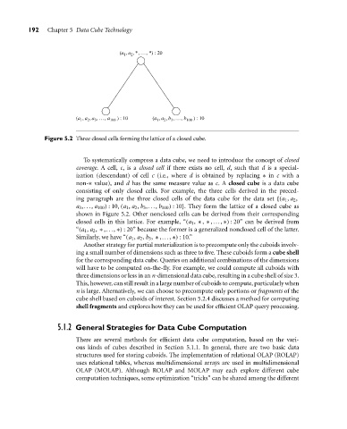
Figure 5.2 Three closed cells forming the lattice of a closed cube.
To systematically compress a data cube, we need to introduce the concept of closed
coverage. A cell, c, is a closed cell if there exists no cell, d, such that d is a special-
ization (descendant) of cell c (i.e., where d is obtained by replacing ∗ in c with a
non-∗ value), and d has the same measure value as c. A closed cube is a data cube
consisting of only closed cells. For example, the three cells derived in the preced-
ing paragraph are the three closed cells of the data cube for the data set {(a 1 , a 2 ,
a 3 ,..., a 100 ) : 10, (a 1 , a 2 , b 3 ,..., b 100 ) : 10}. They form the lattice of a closed cube as
shown in Figure 5.2. Other nonclosed cells can be derived from their corresponding
closed cells in this lattice. For example, “(a 1 , ∗ , ∗ ,..., ∗) : 20” can be derived from
“(a 1 , a 2 , ∗ ,..., ∗) : 20” because the former is a generalized nonclosed cell of the latter.
Similarly, we have “(a 1 , a 2 , b 3 , ∗ ,..., ∗) : 10.”
Another strategy for partial materialization is to precompute only the cuboids involv-
ing a small number of dimensions such as three to five. These cuboids form a cube shell
for the corresponding data cube. Queries on additional combinations of the dimensions
will have to be computed on-the-fly. For example, we could compute all cuboids with
three dimensions or less in an n-dimensional data cube, resulting in a cube shell of size 3.
This, however, can still result in a large number of cuboids to compute, particularly when
n is large. Alternatively, we can choose to precompute only portions or fragments of the
cube shell based on cuboids of interest. Section 5.2.4 discusses a method for computing
shell fragments and explores how they can be used for efficient OLAP query processing.

5.1.2 General Strategies for Data Cube Computation
There are several methods for efficient data cube computation, based on the vari-
ous kinds of cubes described in Section 5.1.1. In general, there are two basic data
structures used for storing cuboids. The implementation of relational OLAP (ROLAP)
uses relational tables, whereas multidimensional arrays are used in multidimensional
OLAP (MOLAP). Although ROLAP and MOLAP may each explore different cube
computation techniques, some optimization “tricks” can be shared among the different