Page 237 - Design for Six Sigma a Roadmap for Product Development

208 Chapter Six

6. The robust design loss function provides a better estimate of the
monetary loss incurred as an FR deviates from its targeted per-
formance value T. A quality loss function can be interpreted as a
means to translate variation and target adjustment to monetary
value. It allows the DFSS team to perform a detailed optimization
of cost by relating design terminology to economical estimates. In
its quadratic version, a quality loss is determined by first finding
the functional limits* T ± FR for the concerned FR. The func-
tional limits are the points at which the design would fail, produc-
ing unacceptable performance in approximately half of the
customer applications. For further loss function literature, please
refer to Chaps. 14 to 16. The expected loss function formulas by FR
type as classified in Fig. 6.14 column 5 are as follows:

2
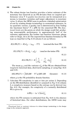
E[L(FR,T)] K[ 2 ( T) ] (nominal-the-best FR)
FR FR
(6.10)
E[L(FR,T)] K( 2 ) (smaller-the-better FR)
2
FR FR
(6.11)
1 3 FR
2
E[L(FR,T)] K (6.12)
2

4
FR FR
The mean FR and the variance 2 of the FR are obtained from
FR
long-term historical data, short-term sampling, or using Eqs. (6.8)
and (6.9).
2
[E[L(FR,T)] Kβ(βM T) g(βM) dM (dynamic) (6.13)
where g is the FR probability density function.
7. Calculate FR complexity in nats or bits per axiom 2. Depending
on the FR distribution identified or assumed in Fig. 6.14 column
5, a complexity measure based on the entropy can be derived (see
Sec. 6.5). For example, the complexity of a normally distributed
FR is given by
h(FR i ) ln 2 e (6.14)
2
FR i
where the FR variance is estimated from Eq. (6.8) in the absence
of historical data. For other distributions, the DFSS team may

*Functional limit or customer tolerance in robust design terminology is the design
range in the axiomatic approach.