Page 351 - Dynamics of Mechanical Systems

0593_C10_fm Page 332 Monday, May 6, 2002 2:57 PM

332 Dynamics of Mechanical Systems

If we multiply the terms of Eq. (10.6.12) by v , the velocity of G in R, we have:
G

⋅
Fv = M a ⋅ v = d  1 M v 2  (10.6.14)
G G G G 
dt  2
Similarly, if we multiply the terms of Eq. (10.6.13) by ωω ωω we have:

0
)⋅+[ ωω
T⋅ωω = I⋅ ( ααωω ×⋅ ( ωω )] ⋅ωω = d  1 ωω I ⋅ ⋅ωω  (10.6.15)
I
dt  2 
By adding the terms of Eqs. (10.6.14) and (10.6.15), we obtain:

⋅
Fv + ⋅ωω = d  1 M v G 2  + d  1 ωω I ⋅ ⋅ωω  (10.6.16)
T
G
dt  2  dt  2 
From Eqs. (10.4.1), (10.4.2), and (10.4.3) we can recognize the left side of Eq. (10.6.16) as
the derivative of the work W of the force system acting on B. Also, from Eq. (10.5.7) we
recognize the right side of Eq. (10.6.16) as the derivative of the kinetic energy K of B.
Hence, Eq. (10.6.16) takes the form:

dW dK
= (10.6.17)
dt dt

Then, by integrating, we have:

W = K − K = ∆ K (10.6.18)
2 1

where, as in Eqs. (10.6.5) and (10.6.10), K and K represent the kinetic energy of B at the
1
2
beginning and end of the time interval that forces are acting on B.
Equations (10.6.5), (10.6.10), and (10.6.18) are expressions of the principle of work and
kinetic energy for a particle, a set of particles, and a rigid body, respectively. Simply stated,
the work done is equal to the change in kinetic energy.
In the remaining sections of this chapter we will consider several examples illustrating
application of this principle. We will also consider combined application of this principle
with the impulse–momentum principles of Chapter 9.

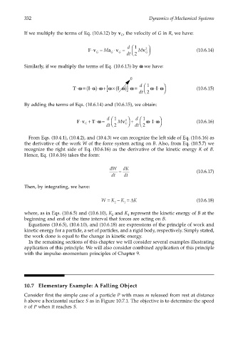
10.7 Elementary Example: A Falling Object
Consider first the simple case of a particle P with mass m released from rest at distance
h above a horizontal surface S as in Figure 10.7.1. The objective is to determine the speed
v of P when it reaches S.