Page 61 - Dynamics of Mechanical Systems

0593_C02_fm Page 42 Monday, May 6, 2002 1:46 PM

42 Dynamics of Mechanical Systems

Similarly, if we express ˆ n 1 , ˆ n 2 , and ˆ n 3 in terms of the ˆ n i , we have:

ˆ n = S n (2.11.7)
i ij j

Observe the difference between Eqs. (2.11.6) and (2.11.7): in Eq. (2.11.6), the sum is taken
over the second index of S , whereas in Eq. (2.11.7) it is taken over the first index. This is
ij
consistent with Eq. (2.11.3), where we see that the first index is associated with the n and
i
the second with the ˆ n i . Observe the same pattern in Eqs. (2.11.6) and (2.11.7).
By substituting from Eqs. (2.11.6) and (2.11.7) into Eqs. (2.11.1) and (2.11.2), we obtain:

ˆ
n = VS ˆ
V = V ˆ i i ij n = V ˆ j (2.11.8)
n
i
j
j
and
ˆ
ˆ
ˆ
V = V i n = VS n = V j n j (2.11.9)
i
j
i ij
Hence, we have:
ˆ
ˆ
V = S V and V = S V (2.11.10)
i ij j i ji j
Observe that Eq. (2.11.10) has the same form as Eqs. (2.11.6) and (2.11.7).
By substituting from Eqs. (2.11.6) and (2.11.7), we obtain the expression:

SS = δ and S S = δ (2.11.11)
ij kj ik ji jk ik
where, as in Eq. (2.6.7), δ is Kronecker’s delta function. In matrix form, this may be
ik
written as:

SS = S S = I or S = S −1 (2.11.12)
T
T
T
where, as before, I is the identity matrix. Hence, S is an orthogonal transformation matrix
(see Eq. (2.10.12)).
ˆ n
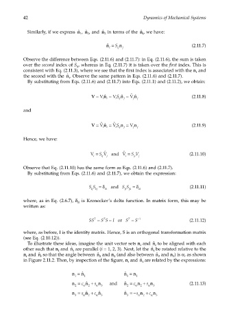
To illustrate these ideas, imagine the unit vector sets n and to be aligned with each
i
i
ˆ n
ˆ n
other such that n and are parallel (i = 1, 2, 3). Next, let the be rotated relative to the
i
i
i
ˆ n
n and so that the angle between ˆ n 2 and n (and also between ˆ n 3 and n ) is α, as shown
i
i
3
2
in Figure 2.11.2. Then, by inspection of the figure, n and are related by the expressions:
ˆ n
i
i
ˆ
n = ˆ n = n
n
1 1 1 1
ˆ
ˆ
n = c n + s n and n = c n + s n (2.11.13)
2 α 2 α 3 2 α 2 α 3
ˆ
ˆ
n = s n + c n ˆ n =−s n + c n
3 α 2 α 3 3 α 2 α 3