Page 224 - Electromagnetics

c
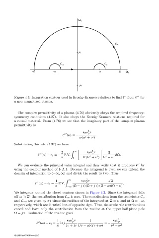
Figure 4.3: Integration contour used in Kronig–Kramers relations to find ˜ from ˜ c for
a non-magnetized plasma.

The complex permittivity of a plasma (4.76) obviously obeys the required frequency-
symmetry conditions (4.27). It also obeys the Kronig–Kramers relations required for
a causal material. From (4.76) we see that the imaginary part of the complex plasma
permittivity is

2
0 ω ν
c p
˜ (ω) =− .
2
2
ω(ω + ν )
Substituting this into (4.37) we have
2
2 ∞ 0 ω ν
p
c
˜ (ω) − 0 =− P.V. − d .
2
2
2
π 0 ( + ν ) − ω 2
We can evaluate the principal value integral and thus verify that it produces ˜ c by
using the contour method of § A.1. Because the integrand is even we can extend the
domain of integration to (−∞, ∞) and divide the result by two. Thus
2
1 ∞ 0 ω ν d
p
c
˜ (ω) − 0 = P.V. .
π −∞ ( − jν)( + jν) ( − ω)( + ω)
We integrate around the closed contour shown in Figure 4.3. Since the integrand falls
4
off as 1/ the contribution from C ∞ is zero. The contributions from the semicircles C ω
and C −ω are given by π j times the residues of the integrand at = ω and at =−ω,
respectively, which are identical but of opposite sign. Thus, the semicircle contributions
cancel and leave only the contribution from the residue at the upper-half-plane pole
= jν. Evaluation of the residue gives
2
1 0 ω ν 1 0 ω 2 p
p
c
˜ (ω) − 0 = 2π j =−
2
π jν + jν ( jν − ω)( jν + ω) ν + ω 2
© 2001 by CRC Press LLC