Page 23 - Electromagnetics

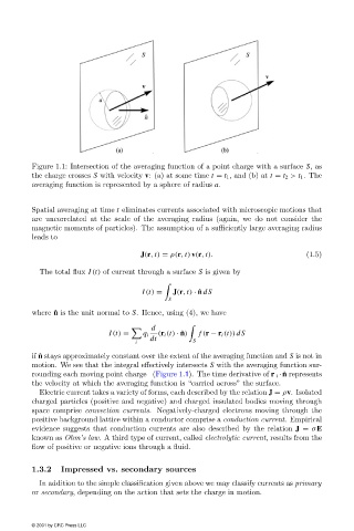
Figure 1.1:Intersection of the averaging function of a point charge with a surface S,as
the charge crosses S with velocity v:(a) at some time t = t 1 , and (b) at t = t 2 > t 1 . The
averaging function is represented by a sphere of radius a.

Spatial averaging at time t eliminates currents associated with microscopic motions that
are uncorrelated at the scale of the averaging radius (again, we do not consider the
magnetic moments of particles). The assumption of a sufficiently large averaging radius
leads to

J(r, t) = ρ(r, t) v(r, t). (1.5)

The total flux I (t) of current through a surface S is given by

I (t) = J(r, t) · ˆ n dS
S
where ˆ n is the unit normal to S. Hence, using (4), we have

d
I (t) = q i (r i (t) · ˆ n) f (r − r i (t)) dS
dt
i S
if ˆ n stays approximately constant over the extent of the averaging function and S is not in
motion. We see that the integral effectively intersects S with the averaging function sur-
rounding each moving point charge (Figure 1.1). The time derivative of r i · ˆ n represents
the velocity at which the averaging function is “carried across” the surface.
Electric current takes a variety of forms, each described by the relation J = ρv. Isolated
charged particles (positive and negative) and charged insulated bodies moving through
space comprise convection currents. Negatively-charged electrons moving through the
positive background lattice within a conductor comprise a conduction current. Empirical
evidence suggests that conduction currents are also described by the relation J = σE
known as Ohm’s law. A third type of current, called electrolytic current, results from the
flow of positive or negative ions through a fluid.

1.3.2 Impressed vs. secondary sources

In addition to the simple classification given above we may classify currents as primary
or secondary, depending on the action that sets the charge in motion.

© 2001 by CRC Press LLC