Page 30 - Electromagnetics

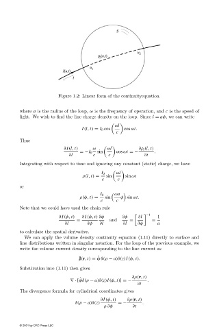
Figure 1.2:Linear form of the continuityequation.

where a is the radius of the loop, ω is the frequency of operation, and c is the speed of
light. We wish to find the line charge density on the loop. Since l = aφ, we can write

ωl
I (l, t) = I 0 cos cos ωt.
c
Thus

∂ I (l, t) ω
ωl ∂ρ l (l, t)
=−I 0 sin cos ωt =− .
∂l c c ∂t
Integrating with respect to time and ignoring any constant (static) charge, we have

I 0 ωl
ρ(l, t) = sin sin ωt
c c
or
I 0 ωa
ρ(φ, t) = sin φ sin ωt.
c c
Note that we could have used the chain rule

∂ I (φ, t) ∂ I (φ, t) ∂φ ∂φ ∂l −1 1
= and = =
∂l ∂φ ∂l ∂l ∂φ a
to calculate the spatial derivative.
We can apply the volume density continuity equation (1.11) directly to surface and
line distributions written in singular notation. For the loop of the previous example, we
write the volume current density corresponding to the line current as

ˆ
J(r, t) = φ δ(ρ − a)δ(z)I (φ, t).
Substitution into (1.11) then gives

∂ρ(r, t)
ˆ
∇· [φδ(ρ − a)δ(z)I (φ, t)] =− .
∂t
The divergence formula for cylindrical coordinates gives
∂ I (φ, t) ∂ρ(r, t)
δ(ρ − a)δ(z) =− .
ρ∂φ ∂t

© 2001 by CRC Press LLC