Page 297 -

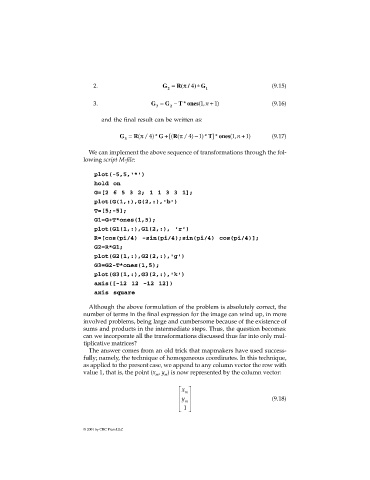
2. G = R( / ) G∗π 4 (9.15)
2 1

3. G = G − T ones* ( ,1 n + )1 (9.16)
3 2
and the final result can be written as:

G = R(/ ) *π 4 G + [( R(/ )π 4 − ) * ]*1 T ones( ,1 n + )1 (9.17)
3

We can implement the above sequence of transformations through the fol-
lowing script M-file:

plot(-5,5,'*')
hold on
G=[2 6 5 3 2; 1 1 3 3 1];
plot(G(1,:),G(2,:),'b')
T=[5;-5];
G1=G+T*ones(1,5);
plot(G1(1,:),G1(2,:), 'r')
R=[cos(pi/4) -sin(pi/4);sin(pi/4) cos(pi/4)];
G2=R*G1;
plot(G2(1,:),G2(2,:),'g')
G3=G2-T*ones(1,5);
plot(G3(1,:),G3(2,:),'k')
axis([-12 12 -12 12])
axis square

Although the above formulation of the problem is absolutely correct, the
number of terms in the final expression for the image can wind up, in more
involved problems, being large and cumbersome because of the existence of
sums and products in the intermediate steps. Thus, the question becomes:
can we incorporate all the transformations discussed thus far into only mul-
tiplicative matrices?
The answer comes from an old trick that mapmakers have used success-
fully; namely, the technique of homogeneous coordinates. In this technique,
as applied to the present case, we append to any column vector the row with
value 1, that is, the point (x , y ) is now represented by the column vector:
m
m
x  
 m 
 y m  (9.18)
  1  

© 2001 by CRC Press LLC