Page 36 -

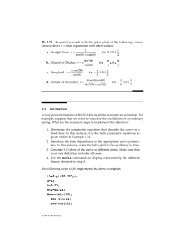
Pb. 1.21 Acquaint yourself with the polar plots of the following curves:
(choose first a = 1, then experiment with other values).

a. Straight lines: r = 1 for 0 ≤≤θ π
cos( )θ + asin( )θ 2
sin ( ) θ π π
2
b. Cissoid of Diocles: r = a for − ≤ ≤
θ
cos( ) θ 3 3
acos(2θ ) π π
c. Strophoid: r = for − ≤ ≤θ
cos( )θ 3 3
a 3 sin( )cos( ) θ π π
θ
θ
d. Folium of Descartes: r = for − ≤ ≤
sin ( ) θ + cos ( ) θ 6 2
3
3

1.9 Animation

A very powerful feature of MATLAB is its ability to render an animation. For
example, suppose that we want to visualize the oscillations of an ordinary
spring. What are the necessary steps to implement this objective?

1. Determine the parametric equations that describe the curve at a
fixed time. In this instance, it is the helix parametric equations as
given earlier in Example 1.14.
2. Introduce the time dependence in the appropriate curve parame-
ters. In this instance, make the helix pitch to be oscillatory in time.
3. Generate 3-D plots of the curve at different times. Make sure that
your axis definition includes all cases.
4. Use the movie commands to display consecutively the different
frames obtained in step 3.

The following script M-file implements the above workplan:

th=0:pi/60:32*pi;
a=1;
A=0.25;
w=2*pi/15;
M=moviein(16);
for t=1:16;
x=a*cos(th);

© 2001 by CRC Press LLC