Page 47 -

from which the difference equation for the area can be deduced:

Ak() = Ak( − 1 ) +    uk() − uk( − 1 ) 3 L 2 2 k

 43
3
(2.17)
2 k−1
= Ak( − 1 ) + 3   2 L 2
24   3
The initial condition for this difference equation is:

A()1 = 3 L 2 (2.18)
49

Clearly, the solution of the above difference equation is the sum of a geo-
metric series, and can therefore be written analytically. For k →∞, this area
has the limit:

Ak( →∞ = 3 L 2 (2.19)
)
20
However, if you did not notice the relationship of the above difference
equation with the sum of a geometric series, you can still solve this equation
numerically, using the following routine and assuming L = 1:

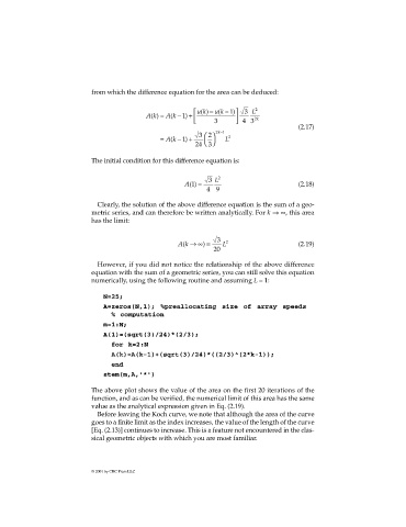
N=25;
A=zeros(N,1); %preallocating size of array speeds
% computation
m=1:N;
A(1)=(sqrt(3)/24)*(2/3);
for k=2:N
A(k)=A(k-1)+(sqrt(3)/24)*((2/3)^(2*k-1));
end
stem(m,A,'*')

The above plot shows the value of the area on the first 20 iterations of the
function, and as can be verified, the numerical limit of this area has the same
value as the analytical expression given in Eq. (2.19).
Before leaving the Koch curve, we note that although the area of the curve
goes to a finite limit as the index increases, the value of the length of the curve
[Eq. (2.13)] continues to increase. This is a feature not encountered in the clas-
sical geometric objects with which you are most familiar.

© 2001 by CRC Press LLC