Page 55 - Elements of Distribution Theory

P1: JZP
052184472Xc02 CUNY148/Severini May 24, 2005 2:29

2.2 Marginal Distributions and Independence 41

Then the marginal density function of X is given by
∞

p X (x) = 6 (1 − x − y)I {x+y<1} dy
0
1−x
2
= 6 (1 − x − y) dy = 3(1 − x) , 0 < x < 1.
0
Since p(x, y)is symmetric in x and y, the marginal density of Y has the same form.

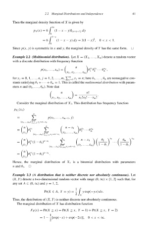
Example 2.2 (Multinomial distribution). Let X = (X 1 ,..., X m ) denote a random vector
with a discrete distribution with frequency function

n
x 1 x 2
x m
p(x 1 ,..., x m ) = θ θ ··· θ ,
1 2 m
x 1 , x 2 ,..., x m
for x j = 0, 1,..., n, j = 1, 2,..., m, m x j = n; here θ 1 ,...,θ m are nonnegative con-
j=1
stants satisfying θ 1 +· · · + θ m = 1. This is called the multinomial distribution with param-
eters n and (θ 1 ,...,θ m ). Note that

n n!
= .
x 1 , x 2 ,..., x m x 1 !x 2 ! ··· x m !
Consider the marginal distribution of X 1 . This distribution has frequency function
(x 1 )
p X 1
n

= p(x 1 ,..., x m−1 , j)
m
(x 2 ,...,x m ): j=2 x j =n−x 1
n
n n − x 1

x 2
= θ x 1 θ ··· θ x m
1 2 m
x 1 m x 2 ,..., x m
(x 2 ,...,x m ): j=2 x j =n−x 1
n
n n − x 1 θ 2 θ m
x 2 x m
x 1
= θ (1 − θ 1 ) n−x 1 ···
1
x 1 m x 2 ,..., x m 1 − θ 1 1 − θ 1
(x 2 ,...,x m ): j=2 x j =n−x 1
n

x 1
= θ (1 − θ 1 ) n−x 1 .
1
x 1
Hence, the marginal distribution of X 1 is a binomial distribution with parameters
n and θ 1 .
Example 2.3 (A distribution that is neither discrete nor absolutely continuous). Let
(X, Y) denote a two-dimensional random vector with range (0, ∞) ×{1, 2} such that, for
any set A ⊂ (0, ∞) and y = 1, 2,
1
Pr(X ∈ A, Y = y) = y exp(−yx) dx.
2 A
Thus, the distribution of (X, Y)is neither discrete nor absolutely continuous.
The marginal distribution of X has distribution function
F X (x) = Pr(X ≤ x) = Pr(X ≤ x, Y = 1) + Pr(X ≤ x, Y = 2)
1
= 1 − [exp(−x) + exp(−2x)], 0 < x < ∞.
2