Page 189 - Engineering Electromagnetics, 8th Edition

CHAPTER 6 Capacitance 171

subject to the charge distribution assumed above,
2
d V 2ρ v0 sech tanh x
x
dx 2 =− a a
in this one-dimensional problem in which variations with y and z are not present. We
integrate once,
dV 2ρ v0 a x
= sech + C 1
dx a
and obtain the electric field intensity,
2ρ v0 a x
E x =− sech − C 1
a
To evaluate the constant of integration C 1 ,we note that no net charge density and no
fields can exist far from the junction. Thus, as x →±∞, E x must approach zero.
Therefore C 1 = 0, and
2ρ v0 a x
E x =− sech (45)
a
Integrating again,
4ρ v0 a 2 −1 x/a
V = tan e + C 2

Let us arbitrarily select our zero reference of potential at the center of the junction,
x = 0,
2
4ρ v0 a π
0 = + C 2
4
and finally,
4ρ v0 a 2 π
e
V = tan −1 x/a − (46)
4
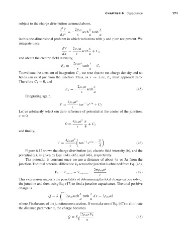
Figure 6.12 shows the charge distribution (a), electric field intensity (b), and the
potential (c), as given by Eqs. (44), (45), and (46), respectively.
The potential is constant once we are a distance of about 4a or 5a from the
junction.Thetotalpotentialdifference V 0 acrossthejunctionisobtainedfromEq.(46),
2πρ v0 a 2
V 0 = V x→∞ − V x→−∞ = (47)

This expression suggests the possibility of determining the total charge on one side of
the junction and then using Eq. (47) to find a junction capacitance. The total positive
charge is

∞ x x
Q = S 2ρ ν0 sech tanh dx = 2ρ ν0 aS
0 a a
where S is the area of the junction cross section. If we make use of Eq. (47) to eliminate
the distance parameter a, the charge becomes

2ρ ν0 V 0
Q = S (48)
π