Page 204 - Engineering Electromagnetics, 8th Edition

186 ENGINEERING ELECTROMAGNETICS

been adjusted so that the addition of this second set of lines will produce an array of
curvilinear squares.
A comparison of Figure 7.4 with the map of the electric field about an infinite
line charge shows that the streamlines of the magnetic field correspond exactly to
the equipotentials of the electric field, and the unnamed (and undrawn) perpendicular
family of lines in the magnetic field corresponds to the streamlines of the electric
field. This correspondence is not an accident, but there are several other concepts
which must be mastered before the analogy between electric and magnetic fields can
be explored more thoroughly.
Using the Biot-Savart law to find H is in many respects similar to the use of
Coulomb’s law to find E. Each requires the determination of a moderately complicated
integrand containing vector quantities, followed by an integration. When we were
concerned with Coulomb’s law we solved a number of examples, including the fields
of the point charge, line charge, and sheet of charge. The law of Biot-Savart can be
used to solve analogous problems in magnetic fields, and some of these problems
appear as exercises at the end of the chapter rather than as examples here.
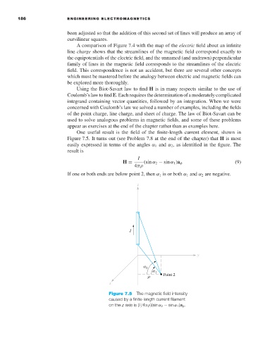
One useful result is the field of the finite-length current element, shown in
Figure 7.5. It turns out (see Problem 7.8 at the end of the chapter) that H is most
easily expressed in terms of the angles α 1 and α 2 ,as identified in the figure. The
result is
I
H = (sin α 2 − sin α 1 )a φ (9)
4πρ
If one or both ends are below point 2, then α 1 is or both α 1 and α 2 are negative.

Figure 7.5 The magnetic field intensity
caused by a finite-length current filament
on the z axis is (I/4πρ)(sin α 2 − sin α 1 )a φ .