Page 240 - Engineering Electromagnetics, 8th Edition

222 ENGINEERING ELECTROMAGNETICS

In order to relate C 1 to the sources in our problem, we may take the curl of A,
∂ A z C 1
∇× A =− a φ =− a φ = B
∂ρ ρ
obtain H,

C 1
H =− a φ
µ 0 ρ
and evaluate the line integral,
2π
C 1 2πC 1
H · dL = I = − a φ · ρ dφ a φ =−
0 µ 0 ρ µ 0
Thus
µ 0 I
C 1 =−
2π
or
µ 0 I b
A z = ln (66)
2π ρ
and
I
H φ =
2πρ
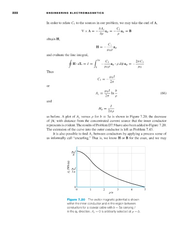
as before. A plot of A z versus ρ for b = 5a is shown in Figure 7.20; the decrease
of |A| with distance from the concentrated current source that the inner conductor
represents is evident. The results of Problem D7.9 have also been added to Figure 7.20.
The extension of the curve into the outer conductor is left as Problem 7.43.
It is also possible to find A z between conductors by applying a process some of
us informally call “uncurling.” That is, we know H or B for the coax, and we may

Figure 7.20 The vector magnetic potential is shown
within the inner conductor and in the region between
conductors for a coaxial cable with b = 5a carrying I
in the a z direction. A z = 0is arbitrarily selected at ρ = b.