Page 50 - Essentials of applied mathematics for scientists and engineers

book Mobk070 March 22, 2007 11:7

40 ESSENTIALS OF APPLIED MATHEMATICS FOR SCIENTISTS AND ENGINEERS

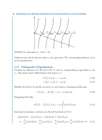
FIGURE 3.4: Eigenvalues of − tan(λ) = Hλ

Solutions exist only for discrete values λ n the eigenvalues. The corresponding solutions X n (x)
are the eigenfunctions.

3.3.1 Orthogonality of Eigenfunctions
Consider two solutions of (3.46) and (3.47), X n and X m corresponding to eigenvalues λ n and
λ m . The primes denote differentiation with respect to x.

(rX ) + qX m =−λ m pX m (3.48)
m

(rX ) + qX n =−λ n pX n (3.49)
n
Multiply the first by X n and the second by X m and subtract, obtaining the following:

(rX n X − rX m X ) = (λ n − λ m )pX m X n (3.50)
m n
Integrating both sides

b

b

r(X X n − X X m ) = (λ n − λ m ) p(x)X n X m dx (3.51)

a
n
m
a
Inserting the boundary conditions into the left-hand side of (3.51)
X (b)X n (b) − X (a)X n (a) − X (b)X m (b) + X (a)X m (a)

n
m
m
n
b 1 a 1 a 1 b 1
=− X m (b)X n (b) + X m (a)X n (a) − X n (a)X m (a) + X m (b)X n (b) = 0 (3.52)
b 2 a 2 a 2 b 2