Page 89 - Essentials of applied mathematics for scientists and engineers

book Mobk070 March 22, 2007 11:7

SOLUTIONS USING FOURIER SERIES AND INTEGRALS 79

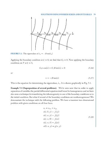
FIGURE 5.1: The eigenvalues of λ n =−B tan(λ n )

Applying the boundary condition at ξ = 0, we find that C 2 = 0. Now applying the boundary
condition on V at ξ = 1,

C 1 λ cos(λ) + C 1 B sin(λ) = 0 (5.26)

or

λ =−B tan(λ) (5.27)

This is the equation for determining the eigenvalues, λ n . It is shown graphically in Fig. 5.1.

Example 5.3 (Superposition of several problems). We’ve seen now that in order to apply
separation of variables the partial differential equation itself must be homogeneous and we have
also seen a technique for transferring the inhomogeneity to one of the boundary conditions or to
the initial condition. But what if several of the boundary conditions are nonhomogeneous? We
demonstrate the technique with the following problem. We have a transient two-dimensional
problem with given conditions on all four faces.

u t = u xx + u yy
u(t, 0, y) = f 1 (y)

u(t, a, y) = f 2 (y)
(5.28)
u(t, x, 0) = f 3 (x)
u(t, x, b) = f 4 (x)

u(0, x, y) = g(x, y)