Page 385 - Excel 2007 Bible

23_044039 ch18.qxp 11/21/06 11:09 AM Page 342
Part II
Working with Formulas and Functions
Using Excel’s Formula Evaluator
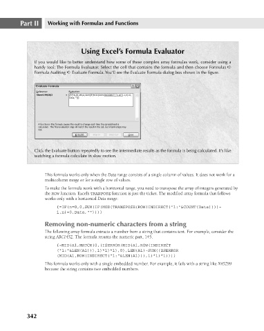
If you would like to better understand how some of these complex array formulas work, consider using a
handy tool: The Formula Evaluator. Select the cell that contains the formula and then choose Formulas ➪
Formula Auditing ➪ Evaluate Formula. You’ll see the Evaluate Formula dialog box shown in the figure.
Click the Evaluate button repeatedly to see the intermediate results as the formula is being calculated. It’s like
watching a formula calculate in slow motion.
This formula works only when the Data range consists of a single column of values. It does not work for a
multicolumn range or for a single row of values.
To make the formula work with a horizontal range, you need to transpose the array of integers generated by
the ROW function. Excel’s TRANPOSE function is just the ticket. The modified array formula that follows
works only with a horizontal Data range:
{=IF(n=0,0,SUM(IF(MOD(TRANSPOSE(ROW(INDIRECT(“1:”&COUNT(Data))))-
1,n)=0,Data,””)))}

Removing non-numeric characters from a string
The following array formula extracts a number from a string that contains text. For example, consider the
string ABC145Z. The formula returns the numeric part, 145.
{=MID(A1,MATCH(0,(ISERROR(MID(A1,ROW(INDIRECT
(“1:”&LEN(A1))),1)*1)*1),0),LEN(A1)-SUM((ISERROR
(MID(A1,ROW(INDIRECT(“1:”&LEN(A1))),1)*1)*1)))}
This formula works only with a single embedded number. For example, it fails with a string like X45Z99
because the string contains two embedded numbers.

342