Page 112 - Excel Workbook for Dummies

11_798452 ch06.qxp 3/13/06 7:48 PM Page 95
Chapter 6: Copying and Correcting Formulas 95
$B$4*12 now appears in the Nper argument text box.
The last required argument is the present value or loan amount for which you
will select cell A7 that is linked to the initial principal entered into cell B2. When
you copy the PMT formula down the rows of column B, you want Excel to adjust
the row number so that it picks and uses the increased principals (that incre-
ment by $1,000 in each subsequent row). You do not, however, want Excel to
adjust the column letter in this argument when you copy the formula to the
columns to the right because all the principals are entered in only one column.
Therefore, for this last PMT argument, you need a mixed cell reference of $A7
(with column reference absolute and row reference relative).
13. With the insertion point in the Pv text box, click cell A7, and then press F4 three
times to convert it to the mixed reference, $A7.
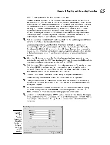
Check the arguments in your Function Arguments dialog box against those
shown in Figure 6-1. When each argument checks out, including the Formula
Result equal to ($1,686.42), proceed to Step 14. If you discover that you need to
change the type of cell reference in any argument, position the insertion pointer
in that reference and press F4 until the correct mixed or absolute reference
appears.
14. Select the OK button to close the Function Arguments dialog box and to com-
plete the formula with the PMT function in cell B7, and then use the Fill handle to
copy this formula down the rows of column B to cell B16.
15. With the range B7:B16 still selected by the cell cursor, use its Fill handle to copy
the original PMT formula across the columns of the table to and including
column G (the entire cell range B7:G16 is selected when you finish copying the
formulas in the second direction across the columns).
16. Use AutoFit to widen columns C:G sufficiently to display their contents.
The results in your loan table should match those shown in Figure 6-2.
17. Change the term from 30 to 15 in cell B4 and note the increase to the monthly
payments in the table, and then use the Undo feature to return the loan term to
its original 30 years.
18. Put Excel into manual recalculation mode and then experiment with changing
the initial principal in cell B2 to 650000 and a starting interest rate in B3 of
2.50%. Press F9 to recalculate the monthly payments in the table.
19. Use Undo to restore the original 400000 and 3% values in cells B2 and B3, respec-
tively, and then save your Loan Payment Table with the filename Solved6-3.xls in
your Chapter 6 folder inside the My Practice Spreadsheets folder. Close the
workbook.

Figure 6-1:
The
Function
Arguments
dialog box
showing the
final argu-
ments for
the PMT
function.