Page 257 - Excel for Scientists and Engineers: Numerical Methods

234 EXCEL NUMERICAL METHODS

The arguments of the function can be entered in other ways. Two of these
are illustrated in rows 12 and 13 of the spreadsheet. If the derivatives are located
in non-adjacent cells, the deriv-formulas argument can be entered as a non-
adjacent selection, as illustrated by the formula in cell J12:
=Runge3(Al l,(Jll,Kll,Ll1),G11:11l,Al2-All,l)

The cell references must be enclosed in parentheses and separated by commas.
The function can also be entered as an array formula, as in cells J 13:L13
{=Runge3(A12, J12:L12,G12:112,A13-A12)}
In this simulation, the largest errors are about 0.05%.

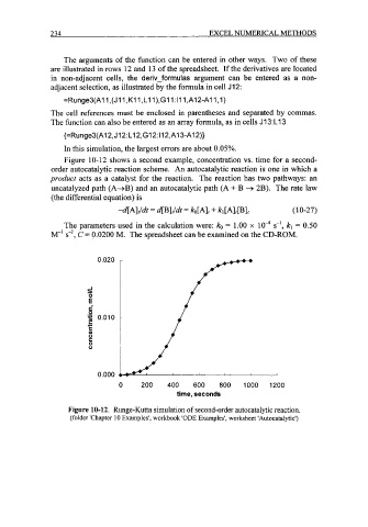
Figure 10-12 shows a second example, concentration vs. time for a second-
order autocatalytic reaction scheme. An autocatalytic reaction is one in which a
product acts as a catalyst for the reaction. The reaction has two pathways: an
uncatalyzed path (A+B) and an autocatalytic path (A + B + 2B). The rate law
(the differential equation) is
4A]t/dt = 4B]t/dt = ko[A]t + kl[Alt[Blt (1 0-27)

The parameters used in the calculation were: ko = 1.00 x lo4 s-I, k, = 0.50
M-' s-', C = 0.0200 M. The spreadsheet can be examined on the CD-ROM.

I
0.020

&
E
E" i
0
'3 0.010 .
E
c
C
0
0
C
0
0
0.000
0 200 400 600 800 1000 1200
time, seconds
Figure 10-12. Runge-Kutta simulation of second-order autocatalytic reaction.
(folder 'Chapter 10 Examples', workbook 'ODE Examples', worksheet 'Autocatalytic')