Page 24 - Fluid-Structure Interactions Slender Structure and Axial Flow (Volume 1)

CONCEPTS, DEFINITIONS AND METHODS 7

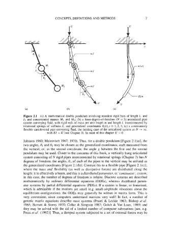
Figure 2.1 (a) A mathematical double pendulum involving massless rigid bars of length I, and
12 and concentrated masses MI and Mz; (b) a three-degree-of-freedom (N = 3) articulated pipe
system conveying fluid, with rigid rods of mass per unit length m and length I, interconnected by
rotational springs of stiffness k, and generalized coordinates Oi(t), i = 1,2, 3; (c) a continuously
flexible cantilevered pipe conveying fluid, the limiting case of the articulated system as N + 00,
with EI = kl (see Chapter 3). In most of this chapter U = 0.
Johnson 1960; Meirovitch 1967, 1970). Thus, for a double pendulum [Figure 2.l(a)], the
two angles, 81 and 8, may be chosen as the generalized coordinates, each measured from
the vertical; or, as the second coordinate, the angle ,y between the first and the second
pendulum may be used. Closer to the concerns of this book, a vertically hung articulated
system consisting of N rigid pipes interconnected by rotational springs (Chapter 3) has N
degrees of freedom; the angles, Oi, of each of the pipes to the vertical may be utilized as
the generalized coordinates [Figure 2.l(b)]. Contrast this to a flexible pipe [Figure 2.l(c)],
where the mass arid flexibility (as well as dissipative forces) are distributed along the
length: it is effectively a beam, and this is a distributedparameter, or ‘continuous’, system;
in this case, the number of degrees of freedom is infinite. Discrete systems are described
mathematically by ordinary differential equations (ODES), whereas distributed param-
eter systems by partial differential equations (PDEs). If a system is linear, or linearized,
which is admissible if the motions are small (e.g. small-amplitude vibrations about the
equilibrium configuration), the ODES may generally be written in matrix form. This is
very convenient, since computers understand matrices very well! In fact, a number of
generic matrix equations describe most systems (Pestel & Leckie 1963; Bishop et al.
1965; Barnett & Storey 1970; Collar & Simpson 1987; Golub & Van Loan, 1989) and
they may be solved with the aid of a limited number of computer subroutines [see, e.g.
Press et al. (1992)l. Thus, a damped system subjected to a set of external forces may be