Page 537 - Fluid-Structure Interactions Slender Structure and Axial Flow (Volume 1)

NONLINEAR DYNAMICS THEORY APPLIED TO A PIPE CONVEYING FLUID 507

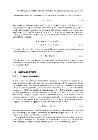
;-dimensional stable one. Following (F.16), the centre manifold is found in the form

with boundary conditions similar to (F.17): h(0,O) = Dh/Du(O, 0) = Dh/Dp(O, 0) = 0.
Consequently, to keep the nonlinear terms cubic in the second of equations (H.2), and to
satisfy the boundary conditions, we must have h be a linear function of u, with ep as a
coefficient, or 'u = ~p[C]u, where [C] here is a j x 1 matrix that has to be determined.
To find [C], an equation similar to (F.20) must be sought, so that the flow on the centre
manifold can be found:
-
u = Eapu + EfI,kuk(EpcU)k

= eapu + €f,.3U3 + O(E2). (H.4)
This means that, to order E, the centre manifold can be approximated as h(u) = 0, and
hence, the flow on the centre manifold can be approximated by
X = AX + f(x, 0). (H.5)

This, of course, is a straighforward operation since one simply has to ignore the stable
component in the equation on the centre, once the original system of equations has been
put in standard form.

H.2 NORMAL FORM

H.2.1 Dynamic instability

In this section, the different manipulations leading to the equation of motion on the
centre manifold are given for the pipe conveying fluid. As will be seen, most of them
are straighfonvard. The different parameters are the same as in Paldoussis & Semler
(1993): the gravity parameter y = 25, the mass parameter fl = 0.2, and the viscoelastic
damping 1y = 0.005. The number of modes is equal to N = 2. It can be shown easily that
for these parameters, a dynamic instability occurs for Qc = 7.093; this, in fact, is also
shown in the computer program, written in MATHEMATICA, which follows. Once the
nonlinear equation of motion is set up, the approximation for the centre manifold is made,
TJ = 0, which corresponds in the program to xg = x4 = 0. Then, the method of averaging
is applied, as outlined in Appendix F. Once the normal form is found,

r = 2.27b.r - 0.31r3, (H.6)

corresponding to equation Out [ 1211 in the listing, the limit-cycle amplitude is computed
and, converting to the original coordinates, the phase-plane plot for p = Q - Qc = 0.3
(shown at the end of the program) is obtained.
The amplitude of the first generalized coordinate, 91, and the frequency of the motion are
given versus p in Figure H.l for another set of parameters: fl = 0.2, y = 10. Agreement
with numerically computed results, especially for p < 0.2, is remarkably good.