Page 298 - Fundamentals of Air Pollution

254 17. The Physics of the Atmosphere

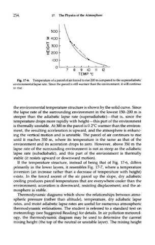
Fig. 17-6. Temperature of a parcel of air forced to rise 200 m compared to the superadiabatic
environmental lapse rate. Since the parcel is still warmer than the environment, it will continue
to rise.

the environmental temperature structure is shown by the solid curve. Since
the lapse rate of the surrounding environment in the lowest 150-200 m is
steeper than the adiabatic lapse rate (superadiabatic)—that is, since the
temperature drops more rapidly with height—this part of the environment
is thermally unstable. At 300 m the parcel is 0.2°C warmer than the environ-
ment, the resulting acceleration is upward, and the atmosphere is enhanc-
ing the vertical motion and is unstable. The parcel of air continues to rise
until it reaches 350 m, where its temperature is the same as that of the
environment and its acceration drops to zero. However, above 350 m the
lapse rate of the surrounding environment is not as steep as the adiabatic
lapse rate (subadiabatic), and this part of the environment is thermally
stable (it resists upward or downward motion).
If the temperature structure, instead of being that of Fig. 17-6, differs
primarily in the lower layers, it resembles Fig. 17-7, where a temperature
inversion (an increase rather than a decrease of temperature with height)
exists. In the forced ascent of the air parcel up the slope, dry adiabatic
cooling produces parcel temperatures that are everywhere cooler than the
environment; acceration is downward, resisting displacement; and the at-
mosphere is stable.
Thermodynamic diagrams which show the relationships between atmo-
spheric pressure (rather than altitude), temperature, dry adiabatic lapse
rates, and moist adiabatic lapse rates are useful for numerous atmospheric
thermodynamic estimations. The student is referred to a standard text on
meteorology (see Suggested Reading) for details. In air pollution meteorol-
ogy, the thermodynamic diagram may be used to determine the current
mixing height (the top of the neutral or unstable layer). The mixing height