Page 44 - Fundamentals of Computational Geoscience Numerical Methods and Algorithms

30 2 Simulating Steady-State Natural Convective Problems

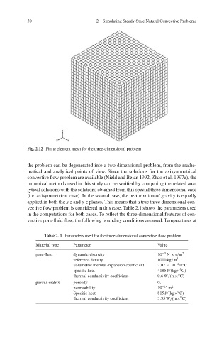
Fig. 2.12 Finite element mesh for the three-dimensional problem

the problem can be degenerated into a two dimensional problem, from the mathe-
matical and analytical points of view. Since the solutions for the axisymmetrical
convective flow problem are available (Nield and Bejan 1992, Zhao et al. 1997a), the
numerical methods used in this study can be verified by comparing the related ana-
lytical solutions with the solutions obtained from this special three dimensional case
(i.e. axisymmetrical case). In the second case, the perturbation of gravity is equally
applied in both the x-z and y-z planes. This means that a true three dimensional con-
vective flow problem is considered in this case. Table 2.1 shows the parameters used
in the computations for both cases. To reflect the three-dimensional features of con-
vective pore-fluid flow, the following boundary conditions are used. Temperatures at

Table 2. 1 Parameters used for the three-dimensional convective flow problem
Material type Parameter Value

pore-fluid dynamic viscosity 10 −3 N × s/m 2
reference density 1000 kg/m 3
−4
volumetric thermal expansion coefficient 2.07 × 10 1/ C
◦
0
specific heat 4185 J/(kg× C)
0
thermal conductivity coefficient 0.6W/(m× C)
porous matrix porosity 0.1
permeability 10 −14 m 2
0
Specific heat 815 J/(kg× C)
0
thermal conductivity coefficient 3.35 W/(m× C)