Page 74 - Fundamentals of Computational Geoscience Numerical Methods and Algorithms

60 3 Algorithm for Simulating Coupled Problems in Hydrothermal Systems

0
v = , 0 T = 25 C ,C 1 = C 2 = C 3 = 0

u =0 u =0
∂T = 0 ∂T = 10km
∂ x ∂ x 0

y

x
0
C 1 = . 0 001 C 2 = . 0 001

v = T , 0 = 225 0 C
10km

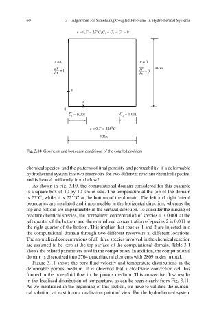
Fig. 3.10 Geometry and boundary conditions of the coupled problem

chemical species, and the patterns of final porosity and permeability, if a deformable
hydrothermal system has two reservoirs for two different reactant chemical species,
and is heated uniformly from below?
As shown in Fig. 3.10, the computational domain considered for this example
is a square box of 10 by 10 km in size. The temperature at the top of the domain
◦
is 25 C, while it is 225 C at the bottom of the domain. The left and right lateral
◦
boundaries are insulated and impermeable in the horizontal direction, whereas the
top and bottom are impermeable in the vertical direction. To consider the mixing of
reactant chemical species, the normalized concentration of species 1 is 0.001 at the
left quarter of the bottom and the normalized concentration of species 2 is 0.001 at
the right quarter of the bottom. This implies that species 1 and 2 are injected into
the computational domain through two different reservoirs at different locations.
The normalized concentrations of all three species involved in the chemical reaction
are assumed to be zero at the top surface of the computational domain. Table 3.1
shows the related parameters used in the computation. In addition, the computational
domain is discretized into 2704 quadrilateral elements with 2809 nodes in total.
Figure 3.11 shows the pore-fluid velocity and temperature distributions in the
deformable porous medium. It is observed that a clockwise convection cell has
formed in the pore-fluid flow in the porous medium. This convective flow results
in the localized distribution of temperature, as can be seen clearly from Fig. 3.11.
As we mentioned in the beginning of this section, we have to validate the numeri-
cal solution, at least from a qualitative point of view. For the hydrothermal system