Page 174 - Fundamentals of Radar Signal Processing

National Weather Service. It is an S-band (3 GHz) system with elevation

and azimuth beamwidths of 0.88º and pulse length in its “short pulse” mode
of τ = 1.57 ms. Suppose the radar measures the RCS in a region of a rain
storm 50 km away as σ = 20 m . Assume the simplified model of the
2
resolution cell volume used to get Eq. (2.25), namely ΔV = (ΔR)(Rθ )(Rϕ )
3
3
2
= ΔR · R θ ϕ . What are the range, azimuth, and elevation resolutions, and
3 3
the resolution cell volume ΔV? What is the volume reflectivity η? Using
Eq. (2.44), compute the value of the meteorological reflectivity factor Z in
3
6
mm /m . Using Table 2.2, how hard is it raining? Note: The value of Z that
6
3
results from Eq. (2.44) will be in m /m = m if wavelength is in meters.
3
3
18
Convert this to units of mm /m by multiplying by 10 before converting to
6
a decibel scale to get dBZ.
9. In terms of wavelengths, by how much must the range between the radar and
a scatterer change in order for the received echo phase to change by 180°?
How far is this at RF frequencies of 1 GHz (L band), 10 GHz (X band),
and 95 GHz (MMW band)?

10. The fourth degree chi-square PDF used to model the case of one dominant
scatterer with many small scatterers is an approximation to the exact model
for this case, which is the non-central chi-square PDF of degree 2. Both
PDFs are listed in Table 2.3 along with the formulas for their variances.

Show that when they both have the same mean , their variances will also
be the same if the non-central chi-square parameter .

11. Suppose a target was modeled as consisting of one large scatterer and many
2
small ones, but that the ratio a of the large scatterer RCS to the sum of the
small scatterer RCS values is 1 (instead of as assumed by the fourth-
degree chi-square model). Assuming the means of the two distributions are
the same, what degree 2m should be chosen for the chi-square so as to

match the variance of the non-central chi-square of degree 2 (See Table
2.3.) Repeat for a = 10. Note: m does not have to be an integer.
2
12. Part of the significance of choosing the probability density function used to
model target RCS (or clutter or other interference) is that the differences in
the “tails” of the PDF can have a significant impact on the probability of
observing relatively large signal values, sometimes called signal “spikes.”
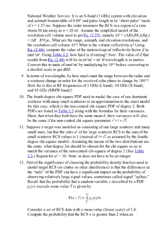
Recall that the probability that a random variable x described by a PDF
p (x) exceeds some value T is given by
x

Consider a set of RCS data with a mean value (linear scale) of 1.0.
Compute the probability that the RCS σ is greater than 2 when an