Page 376 - Fundamentals of Radar Signal Processing

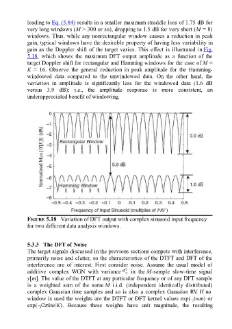
leading to Eq. (5.84) results in a smaller maximum straddle loss of 1.75 dB for

very long windows (M > 300 or so), dropping to 1.5 dB for very short (M = 8)
windows. Thus, while any nonrectangular window causes a reduction in peak
gain, typical windows have the desirable property of having less variability in
gain as the Doppler shift of the target varies. This effect is illustrated in Fig.
5.18, which shows the maximum DFT output amplitude as a function of the
target Doppler shift for rectangular and Hamming windows for the case of M =

K = 16. Observe the general reduction in peak amplitude for the Hamming-
windowed data compared to the unwindowed data. On the other hand, the
variation in amplitude is significantly less for the windowed data (1.6 dB
versus 3.9 dB); i.e., the amplitude response is more consistent, an
underappreciated benefit of windowing.

FIGURE 5.18 Variation of DFT output with complex sinusoid input frequency

for two different data analysis windows.

5.3.3 The DFT of Noise
The target signals discussed in the previous sections compete with interference,
primarily noise and clutter, so the characteristics of the DTFT and DFT of the
interference are of interest. First consider noise. Assume the usual model of
additive complex WGN with variance in the M-sample slow-time signal
y[m]. The value of the DTFT at any particular frequency or of any DFT sample
is a weighted sum of the same M i.i.d. (independent identically distributed)

complex Gaussian time samples and so is also a complex Gaussian RV. If no
window is used the weights are the DTFT or DFT kernel values exp(–jωm) or
exp(–j2πkm/K). Because these weights have unit magnitude, the resulting