Page 243 - gas transport in porous media

239
Chapter 13: Lattice Boltzmann Method
equation, with particle tracking to determine the dispersion in that flow field. The
aperture field between the two plates was determined by filling the gap with a constant
concentration of dye.
For the LB simulation of the Detwiler et al. experiment, a small subset of the
geometry was chosen, mirrored, and replicated in the x-direction after a steady-
state flow field was achieved. Then a slug source was introduced at one end of
the automaton, allowed to disperse downstream, and the method of moments was
∗
used to determine the D . Two 1.54 cm by 1.54 cm subsamples of the real system,
corresponding to 100 × 100 pixels, were used for the LB simulation. This LB size was
picked to contain 35λ, since Detwiler et al. reasoned that at least 20λ was needed to
overcome ergodic effects. This subsample also approximated the width of the initial
solute pulse in the real experiments. Since only the aperture field was known (not
the distribution of porosity along the axis perpendicular to the plates), LB runs were
performed with the aperture symmetrically disposed between the plates, and all on
one side (Figure 13.13 inset).
There were several difficult constraints on the LB model, which deserve mention as
illustrations of limits. First, the experiment was designed to allow reliable determina-
tion of the solute distribution, and to be suitable for Reynolds equation modeling; for
those reasons, the slopes on the textured surface were gentle. Unfortunately, the LB
method for this study used uniform gridding in the x-, y-, and z-directions, so nodes

5000
Symmetric
4500
4000
Asymmetric
3500

3000
D*/Dm 2500

2000
1500
1000
500
0
0 200 400 600 800
Pe
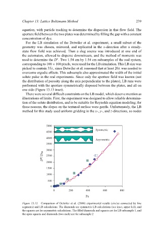
Figure 13.13. Comparison of Detwiler et al. (2000) experimental results (circles connected by line
segments) and LB calculations. The diamonds are symmetric LB calculations (see inset, upper left), and
the squares are for asymmetric calculations. The filled diamonds and squares are for LB subsample 1, and
the open squares and diamonds (two each) are for subsample 2