Page 95 - gas transport in porous media

88
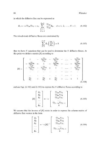
in which the diffusive flux can be expressed as
B=N Whitaker
D Am

J A =−cD Am ∇x A − x A J B , A = 1, 2, ... , N − 1 (6.102)
D AB
B = 1
B = A
The mixed-mode diffusive fluxes are constrained by
A=N
M A

J A = 0 (6.103)
M N
A=1
thus we have N equations that can be used to determine the N diffusive fluxes. At
this point we define a matrix [R] according to

⎡ ⎤
1 − x AD Am − x AD Am − ...... − x AD Am
D AB D AC D AN
⎢ ⎥
⎢ x BD Bm x BD Bm x BD Bm ⎥
⎢ − + 1 − − ...... − ⎥
D BA D BC D BN
⎢ ⎥
⎢ ⎥
⎢ − x CD Cm − x CD Cm + 1 − ...... − x CD Cm ⎥
[R]= ⎢ D CA D CB D CN ⎥
. . . . . − ...... − .
⎢ ⎥
⎢ ⎥
⎢ ⎥
. . . . . − ...... − .
⎢ ⎥
⎣ ⎦
M A M B M C
+ + + ...... + 1
M N M N M N
(6.104)
and use Eqs. (6.102) and (6.103) to express the N diffusive fluxes according to
⎡ ⎤ ⎡ ⎤
J A D Am ∇x A
J B D Bm ∇x B
⎢ ⎥ ⎢ ⎥
⎢ ⎥ ⎢ ⎥
⎢ J C ⎥ ⎢ D Cm ∇x C ⎥
[R] ⎢ ⎥ =−c ⎢ ⎥ (6.105)
... ...
⎢ ⎥ ⎢ ⎥
⎢ ⎥ ⎢ ⎥
⎣ ... ⎦ ⎣ D N−1m ∇x N−1 ⎦
J N 0
We assume that the inverse of [R] exists in order to express the column matrix of
diffusive flux vectors in the form
⎡ ⎤ ⎡ ⎤
J A D Am ∇x A
J B D Bm ∇x B
⎢ ⎥ ⎢ ⎥
⎢ ⎥ ⎢ ⎥
J C D Cm ∇x C
⎢ ⎥ ⎢ ⎥
⎢ ⎥ =−c [R] −1 ⎢ ⎥ (6.106)
⎢ ... ⎥ ⎢ ... ⎥
⎢ ⎥ ⎢ ⎥
⎣ ... ⎦ ⎣ D N−1m ∇x N−1 ⎦
J N 0