Page 472 - Handbook of Biomechatronics

466 Ahmet Fatih Tabak

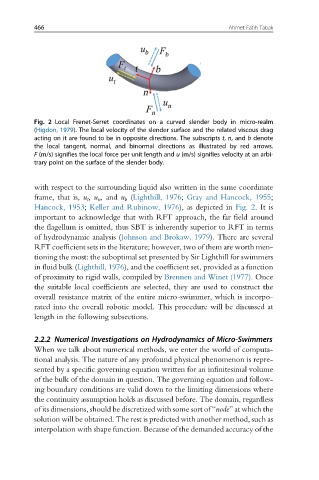
Fig. 2 Local Frenet-Serret coordinates on a curved slender body in micro-realm
(Higdon, 1979). The local velocity of the slender surface and the related viscous drag
acting on it are found to be in opposite directions. The subscripts t, n, and b denote
the local tangent, normal, and binormal directions as illustrated by red arrows.
F (m/s) signifies the local force per unit length and u (m/s) signifies velocity at an arbi-
trary point on the surface of the slender body.

with respect to the surrounding liquid also written in the same coordinate
frame, that is, u t , u n , and u b (Lighthill, 1976; Gray and Hancock, 1955;
Hancock, 1953; Keller and Rubinow, 1976), as depicted in Fig. 2.Itis
important to acknowledge that with RFT approach, the far field around
the flagellum is omitted, thus SBT is inherently superior to RFT in terms
of hydrodynamic analysis (Johnson and Brokaw, 1979). There are several
RFT coefficient sets in the literature; however, two of them are worth men-
tioning the most: the suboptimal set presented by Sir Lighthill for swimmers
in fluid bulk (Lighthill, 1976), and the coefficient set, provided as a function
of proximity to rigid walls, compiled by Brennen and Winet (1977). Once
the suitable local coefficients are selected, they are used to construct the
overall resistance matrix of the entire micro-swimmer, which is incorpo-
rated into the overall robotic model. This procedure will be discussed at
length in the following subsections.

2.2.2 Numerical Investigations on Hydrodynamics of Micro-Swimmers
When we talk about numerical methods, we enter the world of computa-
tional analysis. The nature of any profound physical phenomenon is repre-
sented by a specific governing equation written for an infinitesimal volume
of the bulk of the domain in question. The governing equation and follow-
ing boundary conditions are valid down to the limiting dimensions where
the continuity assumption holds as discussed before. The domain, regardless
of its dimensions, should be discretized with some sort of “node” at which the
solution will be obtained. The rest is predicted with another method, such as
interpolation with shape function. Because of the demanded accuracy of the