Page 348 - High Power Laser Handbook

316 So l i d - S t at e La s e r s Ultrafast Solid-State Lasers 317

Pump laser
8 ps, 100 kHz, 1064 nm
10 W
2.6 W
PCF
Er:Fiber laser DFG Stretcher OPA1
1.6 nJ, 100 MHz, 75 fs 1.05 um-1.55 um 8 ps 32 nJ, 100 kHz 7.4 W
1.55 nm 3.0 um out, 16 pJ positive disp.
Sapphire pulse
compressor
OPA3 OPA2
75 W, 100 kHz, 40 fs 750 uJ, 100 kHz 2.5 uJ, 100 kHz

Pump laser
8 ps, 100 kHz, 1064 nm
100 W
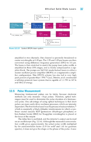
Figure 12.13 Scaled OPCPA laser system.

amplified in two channels. One channel is spectrally broadened to
create wavelengths at 1.05 µm. The 1.55 and 1.05 µm beams are then
converted using difference frequency generation (DFG) to 3.0 µm.
The beam is then stretched to match the pump laser pulse width, is
amplified in three OPA stages, and is finally compressed in a sap-
phire block. The pumps are Nd:YAG mode-locked lasers in either a
master oscillator power amplifier (MOPA) or a regenerative ampli-
fier configuration. This OPCPA scheme has also led to very high
peak powers of greater than 1 PW. Gaul, Ditmire, et al. constructed
35
a tabletop petawatt laser system that is capable of 1.1 PW in 167 fs
and 186 J of energy.

12.5 Pulse Measurement

Measuring femtosecond pulses can be tricky, because electronic
methods can only measure ~10-ps pulses. Therefore, optical tech-
niques must be used to determine the pulse duration of a femtosec-
ond pulse. One advantage of using optical techniques is that short
pulses can more easily drive nonlinear processes, which are intensity
36
dependent. The first method used was the process of autocorrelation,
which is essentially a Mach-Zehnder interferometer in which a non-
linear crystal (usually KDP [potassium dihydrogen phosphate] or
beta barium borate [BBO] for Ti:sapphire wavelengths) is placed at
the focus of the output.
The delay line is oscillated, and the detector’s output can be read
on an oscilloscope (Fig. 12.14). Although the measured autocorrela-
tion width gives approximately the actual pulse width multiplied
2
by the autocorrelation factor (1.55 for sech and 1.41 for gaussian
spectra), it does not give the shape or the phase of the pulse. A new