Page 10 - Human Inspired Dexterity in Robotic Manipulation

4 Human Inspired Dexterity in Robotic Manipulation

Table 1.1 Which statistical test should be performed in each case
Number of Assumption of Assumption
Name of Target elements in Distribution in of variance in
test comparison each group each group each group
T-test Two groups No limitation Nothing Nothing
Tukey- Pairwise No limitation Normal Homogeneity
Kramer differences
Bonferoni/ Pairwise Same Normal Homogeneity
Dunn differences
Scheffe No limitation No limitation Nothing Nothing

1.2.2 State Space Representation

State space representation is conducted when modeling a system as a first-
order differential equation of the input (u), output (y), and state (x). If
the system is linear, the state and observation equations are respectively
represented by

_ x ¼ Ax + Bu
(1.1)
y5Cx + Du
where A, B, C, D are the matrixes. It should be noted that D 5 0 for most of
the cases because it is the feedthrough term. If the system is nonlinear, the
state and observation equations are respectively represented by

_ x ¼ fx, uÞ
ð
(1.2)
y5gx, uÞ
ð
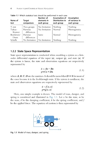
Here, one simple example is shown. The model of mass, damper, and
spring is considered and illustrated in Fig. 1.1. Let x be the state, m be
the mass, d be the damping coefficient, k be the spring coefficient, and f
be the applied force. The equation of motion is then represented by

k
m f

d

x
Fig. 1.1 Model of mass, damper, and spring.