Page 97 - Innovations in Intelligent Machines

UAV Path Planning Using Evolutionary Algorithms 87
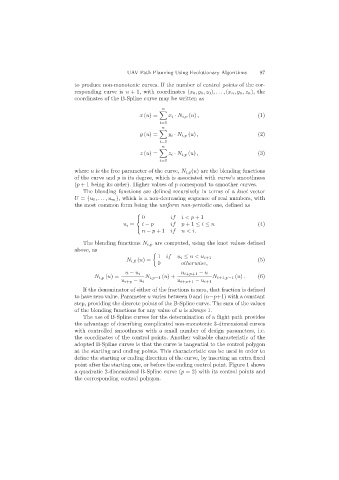
to produce non-monotonic curves. If the number of control points of the cor-
responding curve is n + 1, with coordinates (x 0 ,y 0 ,z 0 ),..., (x n ,y n ,z n ), the
coordinates of the B-Spline curve may be written as

n

x (u)= x i · N i,p (u) , (1)
i=0
n

y (u)= y i · N i,p (u) , (2)
i=0
n

z (u)= z i · N i,p (u) , (3)
i=0
where u is the free parameter of the curve, N i,p (u) are the blending functions
of the curve and p is its degree, which is associated with curve’s smoothness
(p + 1 being its order). Higher values of p correspond to smoother curves.
The blending functions are defined recursively in terms of a knot vector
U = {u 0 ,...,u m }, which is a non-decreasing sequence of real numbers, with
the most common form being the uniform non-periodic one, defined as

⎧
⎨ 0 if i < p +1
u i = i − p if p +1 ≤ i ≤ n (4)
n − p +1 if n < i.
⎩
The blending functions N i,p are computed, using the knot values defined
above, as

1 if u i ≤ u<u i+1
N i,0 (u)= (5)
0 otherwise,
u − u i u i+p+1 − u
N i,p (u)= N i,p−1 (u)+ N i+1,p−1 (u) . (6)
u i+p − u i u i+p+1 − u i+1
If the denominator of either of the fractions is zero, that fraction is defined
to have zero value. Parameter u varies between 0 and (n−p+1) with a constant
step, providing the discrete points of the B-Spline curve. The sum of the values
of the blending functions for any value of u is always 1.
The use of B-Spline curves for the determination of a flight path provides
the advantage of describing complicated non-monotonic 3-dimensional curves
with controlled smoothness with a small number of design parameters, i.e.
the coordinates of the control points. Another valuable characteristic of the
adopted B-Spline curves is that the curve is tangential to the control polygon
at the starting and ending points. This characteristic can be used in order to
define the starting or ending direction of the curve, by inserting an extra fixed
point after the starting one, or before the ending control point. Figure 1 shows
a quadratic 2-dimensional B-Spline curve (p = 2) with its control points and
the corresponding control polygon.