Page 408 - Introduction to AI Robotics

11.4 Dempster-Shafer Theory
1.0 391
don’t know Occupied U don’t know don’t know U
= Occupied
don’t know
0.0 0.4 1.0 = don’t know
Bel
1 Bel
1
occupied don’t know
0.4
0.0 0.6 1.0
Bel don’t know U
2 occupied Occupied U Occupied
Occupied
occupied don’t know = Occupied = Occupied
a.
0.0
occupied don’t know
0.0 0.6 1.0
Bel
2
b.
1.0
don’t know Occupied U don’t know don’t know U
don’t know
= Occupied
Bel 0.6 X 0. 6 = 0.36 = don’t know
1 0.6 X 0. 4 = 0.24
0.0 0.76 1.0
Bel
0.4 3
don’t know U occupied don’t
know
occupied Occupied U Occupied = Occupied d.
Occupied
= Occupied
0.4 X 0. 6 = 0.24 0.4 X 0. 4 = 0.16
0.0
occupied don’t know
0.0 0.6 1.0
Bel
2
c.
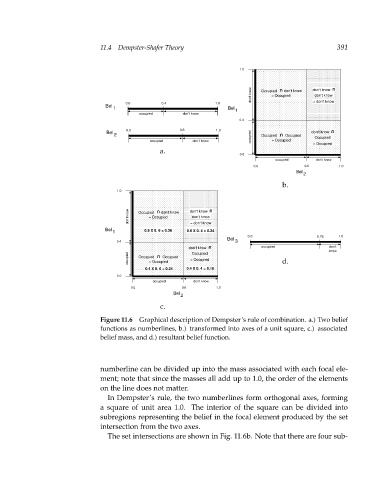
Figure 11.6 Graphical description of Dempster’s rule of combination. a.) Two belief
functions as numberlines, b.) transformed into axes of a unit square, c.) associated
belief mass, and d.) resultant belief function.

numberline can be divided up into the mass associated with each focal ele-
ment; note that since the masses all add up to 1.0, the order of the elements
on the line does not matter.
In Dempster’s rule, the two numberlines form orthogonal axes, forming
a square of unit area 1.0. The interior of the square can be divided into
subregions representing the belief in the focal element produced by the set
intersection from the two axes.
The set intersections are shown in Fig. 11.6b. Note that there are four sub-