Page 432 - Introduction to Information Optics

7.8. Neural Pattern Recognition 4 i /

matching output node. The optimum matching score d c can be defined as

d c(t) 4 j|x(t) - m c(t}\\ = mm{d lk(t)} = min {||x(f) - m /fc (OII}, (7.74)

where c = (I, fc)* represents the node in the output vector space at which a best
match occurred. denotes the Euclidean distance operator.
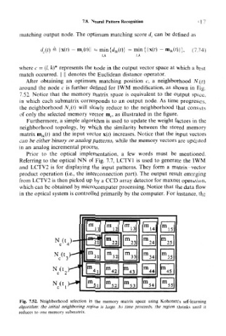
After obtaining an optimum matching position c, a neighborhood N e(t)
around the node c is further defined for IWM modification, as shown in Fig.
7.52. Notice that the memory matrix space is equivalent to the output space,
in which each submatrix corresponds to an output node. As time progresses,
the neighborhood N c(t) will slowly reduce to the neighborhood that consists
of only the selected memory vector m c, as illustrated in the figure.
Furthermore, a simple algorithm is used to update the weight factors in the
neighborhood topology, by which the similarity between the stored memory
matrix m lk(t) and the input vector \(t) increases. Notice that the input vectors
can be either binary or analog patterns, while the memory vectors are updated
in an analog incremental process.
Prior to the optical implementation, a few words must be mentioned.
Referring to the optical NN of Fig. 7.7, LCTV1 is used to generate the IWM
and LCTV2 is for displaying the input patterns. They form a matrix-vector
product operation (i.e., the interconnection part). The output result emerging
from LCTV2 is then picked up by a CCD array detector for maxnet operation,
which can be obtained by microcomputer processing. Notice that the data flow
in the optical system is controlled primarily by the computer. For instance, the

Fig. 7.52. Neighborhood selection in the memory matrix space using Kohonen's self-learning
algorithm: the initial neighboring region is large. As time proceeds, the region shrinks until it
reduces to one memory submatrix.