Page 70 - Lindens Handbook of Batteries
P. 70

ELECTROCHEMICAL PRINCIPLES AND REACTIONS        2.27

                                                                         100
                                                                                                  1
                                                                                            ω max  =
                                                      C dl                                       R ct C dl
                                                                         –Z i /Ω
                                     R s
                                                                                   ω → ∞         ω → 0
                                                                           0
                                                                            0          Z r /Ω         100
                                                    R ct                        R s          R s  + R ct

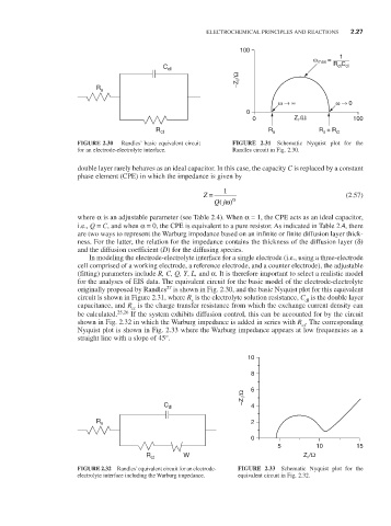
                                FIGURE 2.30   Randles’ basic equivalent circuit   FIGURE  2.31  Schematic  Nyquist  plot  for  the
                                for an electrode-electrolyte interface.  Randles circuit in Fig. 2.30.
                                double layer rarely behaves as an ideal capacitor. In this case, the capacity C is replaced by a constant
                                phase element (CPE) in which the impedance is given by

                                                                Z =  1                              (2.57)
                                                                     ω
                                                                    (
                                                                   Qj ) α
                                where α is an adjustable parameter (see Table 2.4). When α = 1, the CPE acts as an ideal capacitor,
                                i.e., Q = C, and when α = 0, the CPE is equivalent to a pure resistor. As indicated in Table 2.4, there
                                are two ways to represent the Warburg impedance based on an infinite or finite diffusion layer thick-
                                ness. For the latter, the relation for the impedance contains the thickness of the diffusion layer (δ)
                                and the diffusion coefficient (D) for the diffusing species.
                                   In modeling the electrode-electrolyte interface for a single electrode (i.e., using a three-electrode
                                cell comprised of a working electrode, a reference electrode, and a counter electrode), the adjustable
                                (fitting) parameters include R, C, Q, Y, L, and α. It is therefore important to select a realistic model
                                for the analyses of EIS data. The equivalent circuit for the basic model of the electrode-electrolyte
                                                       27
                                originally proposed by Randles  is shown in Fig. 2.30, and the basic Nyquist plot for this equivalent
                                circuit is shown in Figure 2.31, where R  is the electrolyte solution resistance, C  is the double layer
                                                             s
                                                                                          dl
                                capacitance, and R  is the charge transfer resistance from which the exchange current density can
                                              ct
                                be calculated. 25,26  If the system exhibits diffusion control, this can be accounted for by the circuit
                                shown in Fig. 2.32 in which the Warburg impedance is added in series with R . The corresponding
                                                                                         ct
                                Nyquist plot is shown in Fig. 2.33 where the Warburg impedance appears at low frequencies as a
                                straight line with a slope of 45°.
                                                                           10
                                                                            8
                                                                            6
                                                                          –Z i /Ω
                                                      C dl                  4
                                                                            2
                                     R s
                                                                            0
                                                                                   5        10         15
                                                  R ct     W                             Z r /Ω
                                FIGURE 2.32  Randles’ equivalent circuit for an electrode-  FIGURE  2.33  Schematic  Nyquist  plot  for  the
                                electrolyte interface including the Warburg impedance.  equivalent circuit in Fig. 2.32.
   65   66   67   68   69   70   71   72   73   74   75