Page 237 - MATLAB an introduction with applications

222 ——— MATLAB: An Introduction with Applications

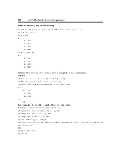
MATLAB Solution [Using built-in function]:

>> A = [12 –6 –6 –1.5; –6 4 3 0.5; –6 3 6 1.5; –1.5 0.5 1.5 1];
>> B = [1;2;3;4];
>> x = A\B
x =
2.7778
4.2222
–0.5556
6.8889
>> x = inv(A)* B
x =
2.7778
4.2222
–0.5556
6.8889

Example E4.7: Solve the set of equations given in Example E4.3. Use Jacobi method.
Solution:
>> A = [3 1 –1; 4 –10 1; 2 1 5]; >> b = [–2 3 4]’;
>> [x,k] = jacobi(A,b,[0 0 0]’,1.e –10)
Jacobi iteration has converged in 38 iterations.
x =
–0.2462
–0.3026
0.9590
k =
38
function [x, k, diff] = jacobi(A,b,x0,tol,kmax)
% Jacobi iteration on the system Ax = b.
if nargin<3, x0 = zeros(size(b));, end
if nargin<4, tol = 1e –10;, end
if nargin<5, kmax = 100;, end
if min(abs(diag(A)))<eps
error(‘Coefficient matrix has zero diagonal entries, iteration cannot be
performed.\r’)
end
[n m] = size(A);
xold = x0;