Page 24 - Machine Learning for Subsurface Characterization

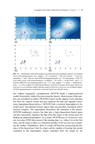
Unsupervised outlier detection techniques Chapter 1 9

FIG. 1.1 Performances of the four unsupervised outlier detection techniques, namely, (A) isolation
forest with hyperparameters: max_samples ¼ 10, n_estimators ¼ 100, max_features ¼ 2, and con-
tamination ¼ “auto”; (B) one-class SVM with hyperparameters: nu ¼ 0.5 and gamma ¼ 0.04; (C)
local outlier factor with hyperparameters: n_neighbors ¼ 20, metric ¼ “minkowiski,” and p ¼ 2;
and (D) DBSCAN with hyperparameters: eps ¼ 0.5, min_samples ¼ 5, metric ¼ “minkowiski,”
and p ¼ 2, on the synthetic two-dimensional dataset containing 25 samples. Red samples (light gray
intheprintversion)indicateoutliers,andbluesamples(darkgrayintheprintversion)indicateinliers.
All other hyperparameters except those mentioned earlier have default values.
few outliers (minimally contaminated). OCSVM builds a representational
model of normality (inliers) by processing the dataset, wherein most of the sam-
ples are considered as inliers. OCSVM is based on the support vector machine
that finds the support vectors and then separates the data into separate classes
using hyperplanes/hyperspheres. OCSVM finds a minimal hypersphere in the
kernel space (transformed feature space) that circumscribes maximum inliers
(normal samples). The hypersphere determines the normality in the dataset.
OCSVM nonlinearly projects the data into a high-dimensional kernel space
and then maximally separates the data from the origin of the kernel space by
finding an optimal hypersphere. As a result, OCSVM may be viewed as a reg-
ular two-class SVM where most of the training data (i.e., inliers) lie in the first
class, and the origin is taken as a dominant member of the second class contain-
ing the outliers. Nonetheless, there is a trade-off between maximizing the dis-
tance of the hyperplane from the origin and the number of training data points
contained in the hypersphere (region separated from the origin by the