Page 203 - Matrices theory and applications

10. Approximation of Eigenvalues
186
2
The algorithm may be rewritten as
1
k
k 0
M x .
x =
k 0
M x
k
We therefore have x =0.
If F = {0},then ρ(M| F ) <ρ(M) by construction. Hence there exist
k
k
(from Theorem 4.2.1) η< ρ(M)and C> 0such that (M| F ) ≤ Cη for
k
k 0
every k.Then (M| F ) z ≤ C 1 η . On the other hand, ρ((M| E ) −1 )=
1/ρ(M), and the same argument as above ensures that (M| E ) −k ≤
k 0
k
k
1/C 2µ ,for some µ ∈ (η, ρ(M)), so that M y ≥ C 3 µ . Hence,
k 0
k 0
M z M y ,
so that
1
k k 0
x ∼ M y .
k 0
M y
0
We are thus reduced to the case where z =0, that is, where M has no
eigenvalue but λ. That will be assumed from now on.
Let r be the degree of the minimal polynomial of M. The vector space
0
0
x contains all the x ’s. Up to
spanned by the vectors x ,Mx ,... ,M r−1 0 k
the replacement of CC n by this linear subspace, one may assume that it
n
equals CC .Thenwehave r = n. Furthermore, since ker(M − λ) n−1 ,a
0
nontrivial linear subspace, is stable under A,wesee that x ∈ ker(M −
λ) n−1 .
n
The vector space CC then admits the basis
0
n
2
1
0
x }.
{v = x ,v =(M − λ)x ,... ,v =(M − λ) n−1 0
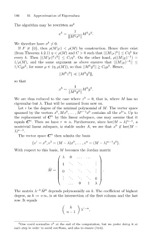
With respect to this basis, M becomes the Jordan matrix
 
λ 0 ... ...
. .
 . . . 
1 . . . . 

 
˜  . . . . . . .  .
. 
M =  0 . . . .
 . . . . 

 . . . . . . . . 0 

... 0 1 λ
The matrix λ −k ˜ k
M depends polynomially on k. The coefficient of highest
degree, as k → +∞, is at the intersection of the first column and the last
row. It equals

k 1−n
λ ,
n − 1
2 k
One could normalize x at the end of the computation, but we prefer doing it at
each step in order to avoid overflows, and also to ensure (10.6).