Page 416 - Matrix Analysis & Applied Linear Algebra

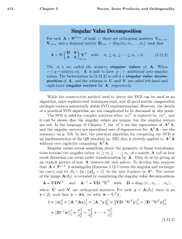
412 Chapter 5 Norms, Inner Products, and Orthogonality

Singular Value Decomposition

m×n
For each A ∈ of rank r, there are orthogonal matrices U m×m ,
V n×n and a diagonal matrix D r×r = diag (σ 1 ,σ 2 ,...,σ r ) such that

D 0 T
A = U V with σ 1 ≥ σ 2 ≥· · · ≥ σ r > 0. (5.12.2)
0 0
m×n
The σ i ’s are called the nonzero singular values of A. When
r< p = min{m, n}, A is said to have p − r additional zero singular
values. The factorization in (5.12.2) is called a singular value decom-
position of A, and the columns in U and V are called left-hand and
right-hand singular vectors for A, respectively.

While the constructive method used to derive the SVD can be used as an
algorithm, more sophisticated techniques exist, and all good matrix computation
packages contain numerically stable SVD implementations. However, the details
of a practical SVD algorithm are too complicated to be discussed at this point.
The SVD is valid for complex matrices when ( ) T is replaced by ( ) , and
∗
it can be shown that the singular values are unique, but the singular vectors
T
2
are not. In the language of Chapter 7, the σ ’s are the eigenvalues of A A,
i
T
and the singular vectors are specialized sets of eigenvectors for A A—see the
summary on p. 555. In fact, the practical algorithm for computing the SVD is
T
an implementation of the QR iteration (p. 535) that is cleverly applied to A A
T
without ever explicitly computing A A.
Singular values reveal something about the geometry of linear transforma-
tions because the singular values σ 1 ≥ σ 2 ≥· · · ≥ σ n of a matrix A tell us how
much distortion can occur under transformation by A. They do so by giving us
an explicit picture of how A distorts the unit sphere. To develop this, suppose
n×n
that A ∈ is nonsingular (Exercise 5.12.5 treats the singular and rectangu-
n
lar case), and let S 2 = {x | x =1} be the unit 2-sphere in . The nature
2
of the image A(S 2 )is revealed by considering the singular value decompositions
A = UDV T and A −1 = VD −1 U T with D = diag (σ 1 ,σ 2 ,...,σ n ) ,
where U and V are orthogonal matrices. For each y ∈ A(S 2 ) there is an
T
x ∈S 2 such that y = Ax, so, with w = U y,

2
y
1= x = A −1 Ax
2 2 = A −1
2 2 = VD −1 U y
2 2 = D −1 U y
2 2

T
T

2

2 w 1 2 w 2 2 w 2 r
w
= D −1
= + + ··· + .

2 σ 2 σ 2 σ 2
1 2 r
(5.12.3)