Page 144 - Mechanics of Asphalt Microstructure and Micromechanics

136 Ch a p t e r Fiv e

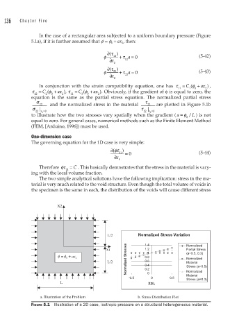
In the case of a rectangular area subjected to a uniform boundary pressure (Figure
5.1a), if it is further assumed that f = f 0 + ax 2 , then:

∂( τ )
φ 12 + τ a = 0 (5-42)
∂x 12
2
∂( τ )
φ 22 + τ a = 0 (5-43)
∂x 22
2
In conjunction with the strain compatibility equation, one has τ = C ( φ + ax ) ,
2
11
1
0
τ = C ( φ + ax ), τ = C ( φ + ax ). Obviously, if the gradient of φ is equal to zero, the
22 2 0 2 12 3 0 2
equation is the same as the partial stress equation. The normalized partial stress
σ τ
22 and the normalized stress in the material 22 are plotted in Figure 5.1b
σ | τ |
22 x = 0 22 x = 0
2
2
to illustrate how the two stresses vary spatially when the gradient ( a = φ / ) is not
L
0
equal to zero. For general cases, numerical methods such as the Finite Element Method
(FEM, [Arduino, 1996]) must be used.
One-dimension case
The governing equation for the 1D case is very simple:
∂(φτ )
11 = 0 (5-44)
∂x
1
Therefore φτ = C . This basically demnstrates that the stress in the material is vary-
11
ing with the local volume fraction.
The two simple analytical solutions have the following implication: stress in the ma-
terial is very much related to the void structure. Even though the total volume of voids in
the specimen is the same in each, the distribution of the voids will cause different stress
X2

L/2 Normalized Stress Variation

Normalized Stresses
1.2
Partial Stress
X1 1.4 Normalized
φ = φ + ax 0.8 1 (a=0.5, 0.3)
0 2 Normalized
L/2 0.6 Material
0.4
Stress (a=0.5)
0.2
Material
-0.5 0 0 0.5 Normalized
Stress (a=0.3)
L X2/L
a. Illustration of the Problem b. Stress Distribution Plot
FIGURE 5.1 Illustration of a 2D case, isotropic pressure on a structural heterogeneous material.