Page 440 - Mechanics of Asphalt Microstructure and Micromechanics

432 C hapter T h ir te en

Molecular Dynamics Simulation

Starting Point

Initial cordinates from lattice Monte Carlo
simulation with initial velocities from
Maxwell-Boltzman distribution
or
continue a previous MD

Calculate Forces Output
Calculate potential function:
⎛ σ 12 σ ⎞ Calculate thermodynamic and
6
r =
V () 4ε ⎜ − 6 ⎟ static system properties:
LJ 12
⎝ r r ⎠ Energies, temperatures, stress…
Calculate force on each particle: If required:
F = ∑ F ij Save coordinates and velocities
save in: <trajectory file>
j
MD loop repeated
every time step
Solve Equations Move Particles
Assign the new coordinates and velocities to
Integrate Newton’s equations
of motion for each particle: each particle through Leapfrog Algorithm:
t Δ
t Δ ⎞
⎛
t Δ ⎞
⎛
i ⎜
i ⎜
dr F vt + ⎟ = v t − ⎟ + F i () t
i = i ⎝ 2 ⎠ ⎝ 2 ⎠ m
dt 2 m ⎛ t Δ ⎞
( +Δ =
t
i rt ) t r () t + Δ ⋅ ⎜ t + ⎟
i
i
⎝ 2 ⎠
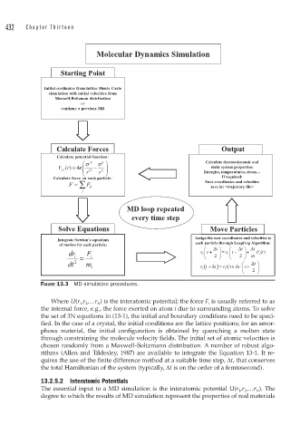
FIGURE 13.3 MD simulation procedures.
Where U(r 1 ,r 2 ,…r N ) is the interatomic potential; the force F i is usually referred to as
the internal force, e.g., the force exerted on atom i due to surrounding atoms. To solve
the set of 3N equations in (13-1), the initial and boundary conditions need to be speci-
fied. In the case of a crystal, the initial conditions are the lattice positions; for an amor-
phous material, the initial configuration is obtained by quenching a molten state
through constraining the molecule velocity fields. The initial set of atomic velocities is
chosen randomly from a Maxwell-Boltzmann distribution. A number of robust algo-
rithms (Allen and Tildesley, 1987) are available to integrate the Equation 13-1. It re-
quires the use of the finite difference method at a suitable time step, Δt, that conserves
the total Hamiltonian of the system (typically, Δt is on the order of a femtosecond).
13.2.5.2 Interatomic Potentials
The essential input to a MD simulation is the interatomic potential U(r 1 ,r 2 ,…r N ). The
degree to which the results of MD simulation represent the properties of real materials