Page 479 - Modelling in Transport Phenomena A Conceptual Approach

10.3. MASS TRANSPORT 459

If 2L/H << 1 and 2L/W << 1, then it is possible to assume that the diffusion
is one-dimensional and postulate that CA = CA(~,Z). In that case, Table C.7 in
Appendix C indicates that the only non-zero molar flux component is NA, and it
is given by
NA, = Jiz = -DAB - (10.3-3)
dCA
dz
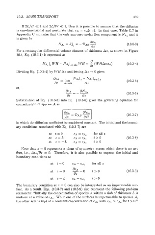
For a rectangular differential volume element of thickness Az, as shown in Figure
10.4, Eq. (10.3-1) is expressed as

(10.3-4)

Dividing Eq. (10.3-4) by WH Az and letting Az --+ 0 gives

(10.3-5)

(10.3-6)

Substitution of Eq. (10.3-3) into Eq. (10.3-6) gives the governing equation for
concentration of species A as

(10.3-7)

in which the diffusion coefficient is considered constant. The initial and the bound-
ary conditions associated with Eq. (10.3-7) are
at t=O CA = CA, for all z
at z=L CA=CA, t >o (10.3-8)
atz=-L CA=CA~ t>O

Note that z = 0 represents a plane of symmetry across which there is no net
flux, i.e., = 0. Therefore, it is also possible to express the initial and
boundary conditions as

at t = 0 CA = CA, for all z

aCA
at z=O -=0 t>O (10.3-9)
az
at z=L CA=CA~ t>O
The boundary condition at z = 0 can also be interpreted as an impermeable sur-
face. As a result, Eqs. (10.3-7) and (10.3-9) also represent the following problem
statement: "Initially the concentration of species A within a slab of thickness L is
uniform at a value of CA,. While one of the surfaces is impermeable to species d,
the other side is kept at a constant concentration of CA, with CA~ > CA, for t > 0."